


Oxford Mathematicians Samuel N. Cohen, Christoph Reisinger and Sheng Wang have developed new methods to help machine learning build economically reasonable models for options markets. By embedding no-arbitrage restrictions within a neural network, more trustworthy and realistic models can be built, allowing for better risk management in the banking system.
"A European call option is a financial contract that gives the buyer the right, but not the obligation, to acquire an underlying asset (e.g. Facebook shares, crude oil) at a specified strike price, denoted as $K$, at a future expiry date, denoted as $T$. As a call option buyer will be guaranteed a non-negative payoff at the option's expiry, the buyer pays a premium for purchasing the option, known as option price and denoted as $C(T,K)$. Banks, funds and many other financial institutions actively trade these options, for the purpose of hedging their risk exposures to the underlying asset or simply speculating on the market. Both the underlying asset price and the option prices change stochastically over time, exposing option traders to considerable market risks. To manage risks of traders' option positions, it is crucial to model joint dynamics of liquid call options and their underlying asset. However, restrictive model specifications expose the risk manager to model risk, the danger of false predictions and erroneous decision making due to inaccurate assumptions on the market behaviour.

Figure 1. The quoted strikes (horizontal axis) for all expiries (vertical axis) of CME weekly- and monthly-listed EURUSD European call options as of 31st May, 2018. Each dot represents a market quote.
In our recent work, we harness advances in neural network methodology and combine them with fundamental economic considerations of options markets to learn a realistic model for the dynamics of options books from observed price time series. The learned model can then be used for generating forward-looking scenarios in the estimation of risk measures of positions or the valuation of more exotic derivative contracts.
Specifically, we consider a financial market where the following assets are liquidly traded: a stock $S$ and a collection of European call options $C(T,K)$ on $S$ with various expiries $T \in \mathcal{T}$ and strikes $K \in \mathcal{K}$ (see Figure 1 as an example). These assets' prices are known to be related to each other in complex ways. For example, the volatility of the stock price which is consistent with the option price of a certain strike and maturity depends on these variables in a characteristic, qualitatively universal way. These stylised relationships suggest that there is significant statistical information captured in the interrelated prices of the stock and options. However, modelling these jointly is challenging. Furthermore, as we detail below, there are various constraints on prices which must hold in the absence of arbitrage, and these should be reflected in any statistical model.
Arbitrage refers to a costless trading strategy that has zero risk and a positive probability of profit. A static arbitrage is an arbitrage exploitable by fixed positions in options and the underlying stock at initial time. As an example, it must hold the condition that $C(T,K_1) \geq C(T,K_2)$ for $K_1 < K_2$, otherwise by buying one $(T, K_1)$ option and selling one $(T, K_2)$ option, we make immediate profit of $C(T, K_2) - C(T, K_1)$ with non-negative terminal payoff. Crucially, this effect is independent of any assumptions on the behaviour of the underlying asset. Another type of arbitrage is called dynamic arbitrage, where positions in options and the underlying stock can change over time; dynamic arbitrage relies on dynamics and path properties of the tradable assets. An economically meaningful model should admit neither type of arbitrage.
We construct a family of factor-based market models, where option prices $C$ are represented by a linear combination of factors $\xi$. Therefore, the factor representation in principle allows exact static calibration, and the joint dynamics of options are straightforwardly available once the dynamics of the factors are specified. The models are then given by a finite system of stochastic differential equations (SDEs) for the factors and the stock price. Importantly, we derive an HJM-type drift condition on the factor SDEs which guarantees freedom from dynamic arbitrage, and the state space of the market factor processes where the models are free from static arbitrage. Since static arbitrage constraints are linear inequalities of option prices, together with linear factor representation, the state space for factors is a convex polytope, defined as the shape formed by an intersection of half spaces. As an example, we take a time series of option and stock prices (simulated from a ground-truth Heston-type stochastic local volatility model) and decode two-dimensional factors from them, where the trajectory of the factors and its statically arbitrage-free state space (light green polygon) are displayed in Figure 2.
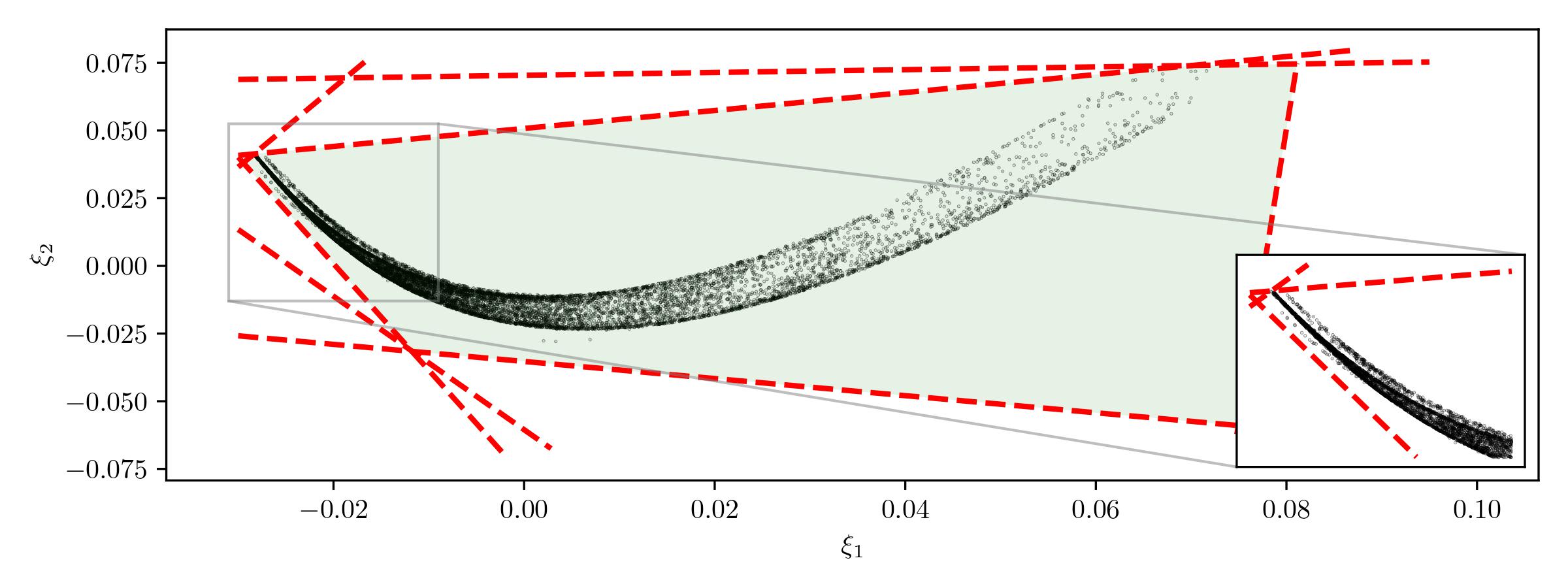
Figure 2: Trajectory (black dots) of the $\mathbb{R}^2$ factors and the corresponding static arbitrage constraints (red dashed lines) projected to the $\mathbb{R}^2$ factor space.
For our models, inference consists of two independent steps: factor decoding and SDE model calibration. The factor decoding step is to extract a smaller number of market factors from prices of finitely many options. These factors are built to reflect the joint goals of eliminating static and dynamic arbitrage in reconstructed prices and guaranteeing statistical accuracy. In the SDE model calibration step, we represent the drift and diffusion functions by neural networks, referred to as neural SDE. By leveraging deep learning algorithms, we train the neural networks by maximising the likelihood of observing the factor paths, subject to the derived arbitrage constraints. This allows for calibration and model selection to be done simultaneously.
No-arbitrage conditions are embedded as part of model inference. Specifically, static arbitrage constraints are characterised by a convex polytope state space for the latent factors; we identify sufficient conditions on the drift and diffusion to restrict the factors to their arbitrage-free domain. Consequently, the neural network that is used to parameterise the drift and diffusion functions needs to be constrained. We propose a novel hard constraint approach that modifies the network to respect sufficient conditions on the drift and diffusion to restrain the process within the polytope. The architecture of the modified neural network is plotted in Figure 3.
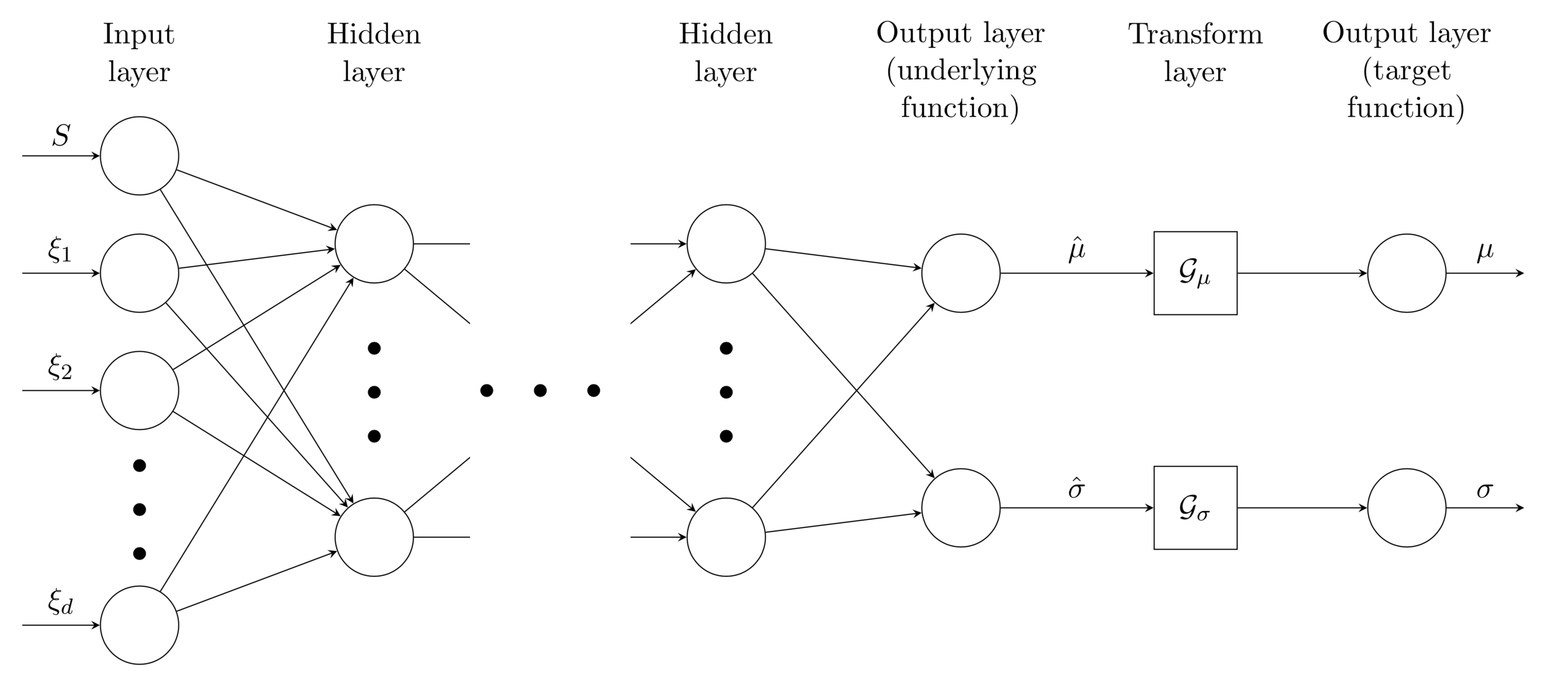
Figure 3. Constrained neural network. The operators $\mathcal{G}_\mu$ and $\mathcal{G}_\sigma$ transform drift and diffusion functions, respectively, such that the resulting process is restrained within the statically arbitrage-free polytope.
As a demonstration of how well the neural network can learn the factor dynamics as shown in Figure 2, we take the learnt model and simulate time series of the two-dimensional factors. In Figure 4, we compare the empirical distributions of the simulated $\xi_1$ and $\xi_2$ with those of the input data (simulated from a Heston-SLV model).

Figure 4. Comparison of the marginal and joint distributions of the simulated $\xi_1$ and $\xi_2$ with the real distributions (generated from the Heston-SLV model).
We see that the learnt model is capable of generating realistic long time series data that are similar to the input data. Through the linear factor representation, it is straightforward to compute call option prices, and indeed prices of other derivatives such as the CBOE VIX volatility index, from the simulated factors. In Figure 5, we plot the simulated time series of VIX and log-return of $S$. We see several occurrences of volatility clustering in the return series, which always coincide with high VIX values.
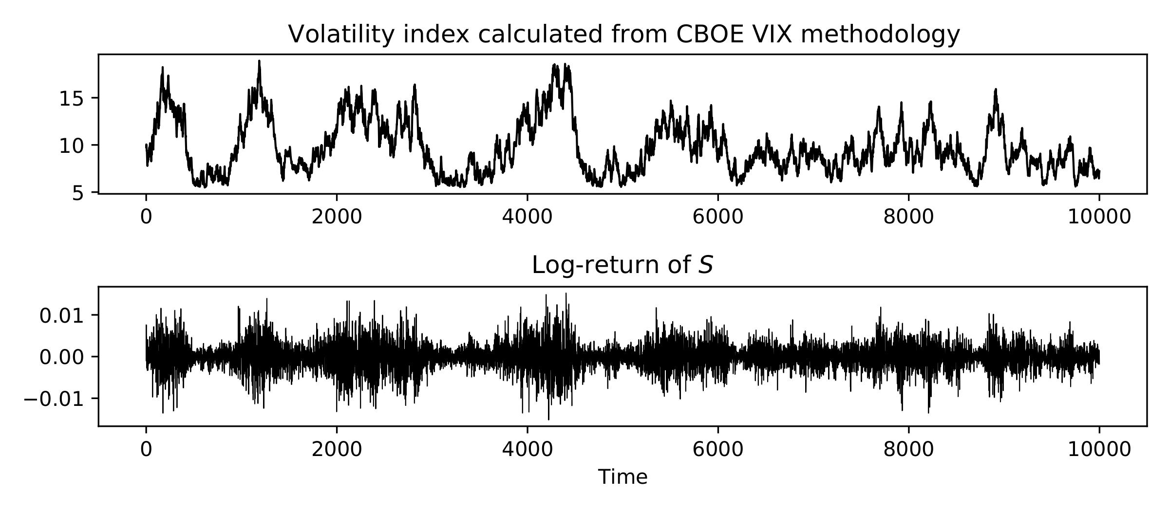
Figure 5. Simulated time series of the VIX volatility index, together with log-returns of the underlying stock.
In conclusion, we construct market models for the stock and options that permit no arbitrage, allow exact cross-sectional calibration, and reflect stylised facts observed from market price dynamics. Importantly, it is practically convenient to estimate these models, given that observations are discrete time series of prices for a large but finite collection of options. In particular, we exploit the recent successes in the use of neural networks as function approximators in order to give a flexible class of models."
This project was supported by CME Group through the Centre for Doctoral Training in Industrially Focused Mathematical Modelling.
[1] S. N. Cohen, C. Reisinger, and S. Wang. Arbitrage-free neural-SDE market models, 2021