

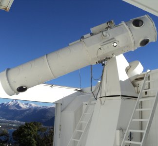
The Sun has been emitting light and illuminating the Earth for more than four billion years. By analyzing the properties of solar light we can infer a wealth of information about what happens on the Sun. A particularly fascinating (and often overlooked) property of light is its polarization state, which characterizes the orientation of the oscillation in a transverse wave. By measuring light polarization, we can gather precious information about the physical conditions of the solar atmosphere and the magnetic fields present therein. To infer this information, it is important to confront observations with numerical simulations. In this brief article we will focus on the latter.
The transfer of partially polarized light is described by the following linear system of first-order coupled inhomogeneous ordinary differential equations (ODEs) \begin{equation} \frac{\rm d}{{\rm d} s}\mathbf I(s) = -\mathbf K(s)\mathbf I(s) + \boldsymbol{\epsilon}(s)\,. \label{eq:RTE} \end{equation}
In this equation, the symbol $s$ is the spatial coordinate measured along the ray under consideration, $\mathbf{I}$ is the Stokes vector, $\mathbf{K}$ is the propagation matrix, and $\boldsymbol{\epsilon}$ is the emission vector.
The analytic solution of this system of ODEs is known only for very simple atmospheric models, and in practice it is necessary to solve the above equation by means of numerical methods.
Although the system of ODEs in the equation above is linear, which simplifies the analysis, the propagation matrix $\mathbf{K}$ depends on the spatial coordinate $s$, which implies that this system is nonautonomous. Additionally, it exhibits stiffness, which means that extra care must be taken into account to compute a numerical solution because numerical instabilities are just around the corner, and these have the potential to completely invalidate numerical computations.
In their work Oxford Mathematician Alberto Paganini and Gioele Janett from the solar research institute IRSOL in Locarno, Switzerland, have developed a new algorithm to solve the equation above. This algorithm is based on a switching mechanism that is capable of noticing when stiffness kicks in. This allows combining stable methods, which are computationally expensive and are used in the presence of stiffness, with explicit methods, which are computationally inexpensive but of no-use when stiffness arises.
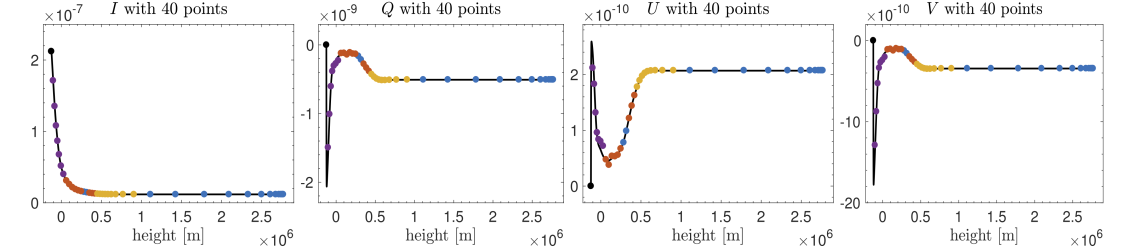
The following plots display the evolution of the Stokes components along the vertical direction for the Fe I line at 6301.50 Å in the proximity of the line core frequency (the Stokes profiles have been computed considering a one-dimensional semi-empirical model of the solar atmosphere, discretized on a sequence of increasingly refined grids). The black line depicts the reference solution, while the dots denote the numerical solution obtained with the new algorithm. Different dot colors correspond to different methods: Blue dots indicate the use of an explicit method, whereas yellow, orange, and purple dots indicate the use of three variants of stable methods (each triggered by a different degree of instability). These pictures (below) show that the algorithm is capable of switching and choosing the appropriate method whenever necessary and of delivering good approximations of the equation above.
This research has been published in The Astrophysical Journal, Vol 857, Number 2, p. 91 (2018).