Oxford Mathematician Markus Dablander talks about his collaboration with Julius Berner and Philipp Grohs from the University of Vienna. Together they developed a new deep-learning-based method for the computationally efficient solution of high-dimensional parametric Kolmogorov PDEs.
"Kolmogorov PDEs are linear parabolic partial differential equations of the form \begin{equation*} \label{kol_pde_intro} \tfrac{\partial u_\gamma }{\partial t} = \tfrac{1}{2} \text{Trace}\big(\sigma_\gamma [\sigma_\gamma ]^{*}\nabla_x^2 u_\gamma \big) + \langle \mu_\gamma , \nabla_x u_\gamma \rangle, \quad u_\gamma (x,0) = \varphi_\gamma(x). \end{equation*} The functions \begin{equation*}\varphi_\gamma : \mathbb{R}^d \rightarrow \mathbb{R} \quad \text{(initial condition)}, \quad \sigma_\gamma : \mathbb{R}^d \rightarrow \mathbb{R}^{d \times d}, \quad \mu_\gamma : \mathbb{R}^d \rightarrow \mathbb{R}^{d} \quad \text{(coefficient maps)}, \end{equation*} are continuous, and are implicitly determined by a real parameter vector $\gamma \in D $ whereby $D$ is a compact set in Euclidean space. Equations of this type represent a broad class of problems and frequently appear in practical applications in physics and financial engineering. In particular, the heat equation from physical modelling as well as the widely-known Black-Scholes equation from computational finance are important special cases of Kolmogorov PDEs.
Typically, one is interested in finding the (viscosity) solution \begin{equation*} u_\gamma : [v,w]^d \times [0,T] \rightarrow \mathbb{R} \end{equation*} of a given Kolmogorov PDE on a predefined space-time region of the form $[v,w]^{d} \times [0,T]$. In almost all cases, however, Kolmogorov PDEs cannot be solved explicitly. Furthermore, standard numerical solution algorithms for PDEs, in particular those based on a discretisation of the considered domain, are known to suffer from the so-called curse of dimensionality. This means that their computational cost grows exponentially in the dimension of the domain, which makes these techniques unusable in high dimensions. The development of new, computationally efficient methods for the numerical solution of Kolmogorov PDEs is therefore of high interest for applied scientists.
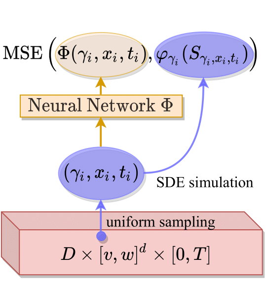
We were able to develop a novel deep learning algorithm capable of efficiently approximating the solutions $(u_\gamma )_{\gamma \in D}$ of a whole family of potentially very high-dimensional $\gamma$-parametrised Kolmogorov PDEs on a full space-time region. Specifically, our proposed method allows us to train a single deep neural network \begin{equation*} \Phi\colon D \times [v,w]^d \times [0,T] \rightarrow \mathbb{R} \end{equation*} to approximate the parametric solution map \begin{align*} \label{eq:gen_sol_map} \bar{u} : D \times [v,w]^d \times [0,T] \rightarrow \mathbb{R}, \quad (\gamma, x, t) \mapsto \bar{u}(\gamma, x, t) := u_\gamma (x,t), \end{align*} of a family of $\gamma$-parametrized Kolmogorov PDEs on the generalised domain $D \times [v,w]^d \times [0,T]$. The key idea of our novel algorithm is to reformulate the parametric solution map $\bar{u}$ of the $\gamma$-parametrized Kolmogorov PDE as the regression function of an appropriately chosen supervised statistical learning problem. This reformulation is based on an application of the so-called Feynman-Kac formula, which links the theory of linear parabolic PDEs to the theory of stochastic differential equations via $$ \bar{u}(\gamma,x,t) = \mathbb{E}[\varphi_{\gamma}(S_{\gamma,x,t})]. $$ Here $S_{\gamma,x,t}$ is the solution of an associated $\gamma$-parametrised stochastic differential equation with starting point $x$ at time $t$: $$ dS_{\gamma,x,t} = \mu_\gamma (S_{\gamma,x,t}) dt + \sigma_\gamma (S_{\gamma,x,t}) dB_t, \quad S_{\gamma,x,0} = x. $$ The resulting stochastic framework can be exploited to prove that $\bar{u}$ must be the solution of a specifically constructed statistical learning problem. Realisations of the predictor variable of this learning problem can be simulated by drawing uniformly distributed samples of the domain $(\gamma_i, x_i, t_i) \in D \times [v,w]^d \times [0,T]$ while realisations of the dependent target variable can be generated by simulating realisations $\varphi_{\gamma_i}(s_{\gamma_i, x_i, t_i})$ of $\varphi_{\gamma_i}(S_{\gamma_i, x_i, t_i})$. Thus, a potentially infinite amount of independent and identically distributed training points can be simulated by solving for $S_{\gamma_i, x_i, t_i}$ via simple standard numerical techniques such as the Euler-Maruyama scheme. The simulated predictor-target-pairs $((\gamma_i, x_i, t_i) ,\varphi_{\gamma_i}(s_{\gamma_i, x_i, t_i}))$ can then be used to train the deep network $\Phi$ to approximate the solution $\bar{u}.$ An illustration of this training workflow is depicted in the figure below.
We mathematically investigated the approximation and generalisation errors of our constructed learning algorithm for important special cases and discovered that, remarkably, it does not suffer from the curse of dimensionality. In addition to our theoretical findings, we were able to also observe numerically that the computational cost of our our proposed technique does indeed grow polynomially rather than exponentially in the problem dimension; this makes very high-dimensional settings computationally accessible for our method.
Our work was accepted for publication at the 2020 Conference on Neural Information Processing Systems (NeurIPS). A preprint can be accessed here.
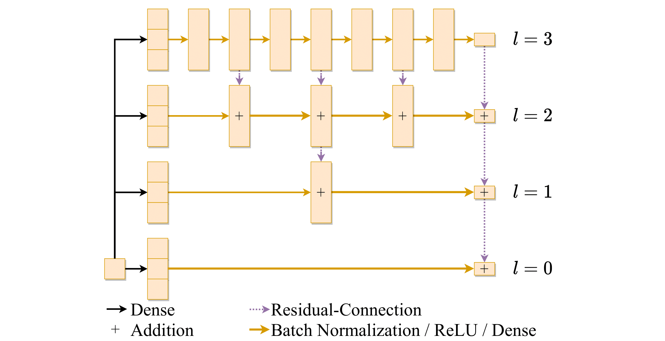
Below is a picture of the Multilevel architecture we used for our deep network $\Phi$ (click to enlarge)."