Season 3 Episode 3

In this episode, Lucy joins the livestream to demonstrate something she's learning at university; Double Integration.
Further Reading
Area at A-level
At A-level (or equivalent), you learn that the area “under” a curve $y=f(x)$ (where “under” means the area between this curve and the $x$-axis) between $x=a$ and $x=b$ with $a<b$ is given by
\[ \int_a^b f(x)\,\mathrm{d}x.\]
Integration is quite similar to summation (adding), and one interpretation of this equation is “we’re adding together lots of little rectangles, and each rectangle has tiny width $\mathrm{d}x$ and height $f(x)$ which depends on $x$”.
If $f(x)$ is a power of $x$ like $f(x)=x^{n}$, then at A-level you learn that $\int_a^b x^n \,\mathrm{d}x=\frac{1}{n+1}b^{n+1}-=\frac{1}{n+1}a^{n+1}$ so long as $n\neq 1$.
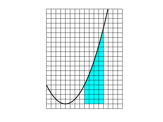
Exercise: if you’ve just learned this fact by reading it here, try to use it to work out the area of the region bounded by the line $x=1$ on the left, the line $x=2$ on the right, the $x$-axis below, and the curve $y=x^2$ above. If you draw the curve $y=x^2$ on squared paper then you can check your answer (sort of) by counting squares to estimate the area. The image shows my attempt at doing this!

Area at University
At university, we can take this one step further – how about instead of thinking about adding together rectangles of height $f(x)$ and width $\mathrm{d}x$, we think about adding together tiny little squares or rectangles with height $\mathrm{d}y$ and width $\mathrm{d}x$. This is a lot like the method above for estimating areas by counting the grid squares inside the region!
Each little region has area $\mathrm{d}x\mathrm{d}y$. In the livestream we sometimes wrote that as $1\mathrm{d}x\mathrm{d}y$ just to remember that there isn’t anything else like an $f(x)$ there!
We can add up the areas first across different values of $y$ and then across different values of $x$. That gives us something like
\[\int_{x=a}^{x=b} \int_{y=f(x)}^{y=g(x)} 1 \mathrm{d}y\mathrm{d}x.\]
Notice that the limits for $y$ are allowed to be functions of $x$, which we’ll then deal with when we do the integration over $x$. But the outside limits for $x$ have to be numbers because at that point we’ve integrated $y$ out of the problem, so to get an actual number at the end, rather than something weird like a function of $y$, we need some numbers for the limits here. The strength here is that it lets us find the area between two curves $f(x)$ and $g(x)$ with $g(x)>f(x)$; this is so useful that some people on A-level courses even learn the fact that it’s
\[\int_{x=a}^{x=b} g(x)-f(x) \mathrm{d}y\mathrm{d}x.\]
Notice that this is precisely what we get if we do the $y$-integral in the previous expression (the integral of $1$ with respect to $y$ is $y$ and then we plug in the limits $g(x)$ and $f(x)$).
Even better though, we have the option to add together the little regions $\mathrm{d}x\mathrm{d}y$ by first adding “sideways”; integrating with respect to $x$ first, to find the area of a wide short rectangle from the left of our region to the right. Then we’ll integrate with respect to $y$ to add up the areas of those rectangles. The notation for this is something like
\[\int_{y=c}^{y=d} \int_{x=p(y)}^{x=q(y)} 1 \mathrm{d}x\mathrm{d}y.\]
That’s a lot to take in! I’ve used the letters $p$ and $q$ for two functions of $y$ on the limits for $x$; in this sideways world, we’re first integrating from left to right, and the start and stop points are allowed to depend on $y$. It would perhaps be more normal to call those two functions $f$ and $g$, but I want to really make the point that these are different functions from the ones that we had before. The reasoning here is once again that it’s OK for things inside the $y$-integral to depend on $y$ (even the limits of the inside integral!), but it’s not OK for things outside the $x$-integral to depend on $x$ - that’s why the limits for $y$ are just numbers $c$ and $d$ here (it would perhaps be more normal to just call them $a$ and $b$ again, but they’re not the same $a$ and $b$ as before!)
This lets us do cool things like finding the area between the curve $y=\sqrt{x}$, the $y$-axis, and the lines $y=0$ and $y=2$. We would write down something like
\[\int_{y=0}^{y=2} \int_{x=0}^{x=y^2} 1 \mathrm{d}x\mathrm{d}y.\]
Notice that I’ve had to rearrange the equation $y=\sqrt{x}$ into an equation for $x$. Let’s do the integrals! The first thing is to integrate just 1 with respect to $x$. Easy, that’s just $x$, and I can plug in the limits (because I rearranged them!) to get
\[\int_{y=0}^{y=2} y^2\mathrm{d}y.\]
Now I just need to integrate $y^2$ with respect to $y$ from $0$ to $2$; I can do that! I get $\frac{8}{3}$.
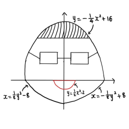
Find the area of my face
On the livestream, Lucy challenged you to find the area of my face bounded by the following curves;
$y=-\frac{1}{4}x^2+16$ between $x=-2$ and $x=2$,
$x=\frac{1}{8}y^2-8$ between $y=-1$ and $y=0$
$x=-\frac{1}{8}y^2+8$ between $y=-1$ and $y=0$
Remember to subtract the area of my smile, which is bounded by the $x$-axis and the curve $y=\frac{1}{2}x^2-2$.

Probability
On the livestream we worked out the average (absolute) difference between two fair six-sided dice. We made a table like this;
| First die \ Second die | 1 | 2 | 3 | 4 | 5 | 6 |
| 1 | 0 | 1 | 2 | 3 | 4 | 5 |
| 2 | 1 | 0 | 1 | 2 | 3 | 4 |
| 3 | 2 | 1 | 0 | 1 | 2 | 3 |
| 4 | 3 | 2 | 1 | 0 | 1 | 2 |
| 5 | 4 | 3 | 2 | 1 | 0 | 1 |
| 6 | 5 | 4 | 3 | 2 | 1 | 0 |
And we worked out that the total of those numbers is 70, so the average is $\frac{35}{18}$. If you didn’t try this, you could check the sum now.
I can think of several ways to do that sum! One of the quickest ways I’ve found works like this;
- The diagonal is full of zeros. The numbers above the diagonal are the same as the numbers below the diagonal.
- Above the diagonal, each row sums to a triangle number
- The sum of consecutive triangles numbers is a tetrahedral number (the fourth diagonal of Pascal’s triangle!) and there’s a formula for those.
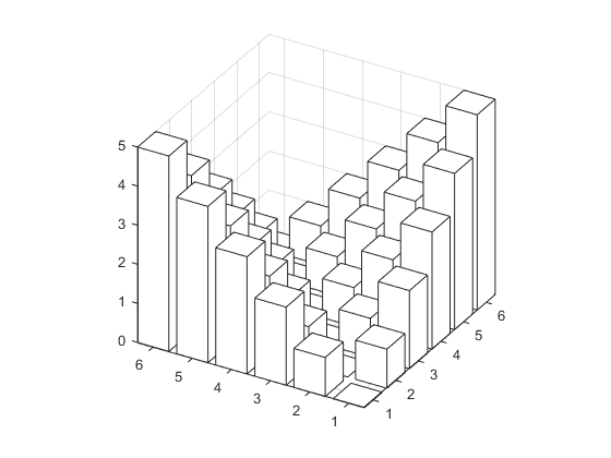
This method also generalises to other size dice (with other numbers of faces). I thought of tetrahedrons because I thought about visualising the numbers in the grid by stacking the corresponding number of cubes on top of each grid square in the table – that makes a pair of tetrahedra like a sort of valley shape.

We also did some integrals to work out what the average (absolute) difference between two fair random numbers is – taking our random numbers to be uniformly distributed between 0 and 1. This is a sort of continuous version of the sum above. The answer turns out to be 1/3. We can compare that with our result for six-sided dice if we remember that the numbers on a six-sided dice go up to six, so it makes sense for the average difference to be about six times as big as the continuous random variable example, where the numbers only go up to 1.
Advantageous Probability
Here’s a different probability question. If I roll two six-sided dice and take the larger number, what do you expect that larger number to be? Clearly it’s a bit bigger than 3.5 (because that’s the average result for just one die), but I’m not aware of a simple argument that explains how much bigger than 3.5 it should be.
The process of rolling two dice and taking the higher number is called “rolling with advantage” in Dungeons and Dragons.
The best way that I know to attack this problem is to make a table again.
| First die \ Second die | 1 | 2 | 3 | 4 | 5 | 6 |
| 1 | 1 | 2 | 3 | 4 | 5 | 6 |
| 2 | 2 | 2 | 3 | 4 | 5 | 6 |
| 3 | 3 | 3 | 3 | 4 | 5 | 6 |
| 4 | 4 | 4 | 4 | 4 | 5 | 6 |
| 5 | 5 | 5 | 5 | 5 | 5 | 6 |
| 6 | 6 | 6 | 6 | 6 | 6 | 6 |
Now we’ve got a sum to do. There are different ways to do it. My first idea was to write down $1\times 1+3\times 2+5\times 3+7\times 4+9\times 5+11\times 6$. If you do that then you find out that the sum is 161. It’s also possible to generalise that to $n$-sided dice if you can spot the pattern to the general term in that sum, and if you know that the sum of the first $n$ square numbers is $\frac{(2n+1)n(n+1) }{6}$. Generalising this might be handy if you care about 20-sided dice for some reason.
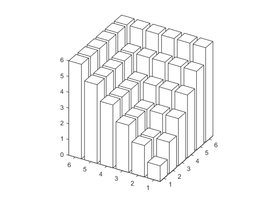
But then I thought about visualising this like we did with the tetrahedra above, and that gave me a new idea about how to do this sum.

I don’t know about you, but when I look at that picture, I see a big cube with something cut out of it. If I think about filling in the gaps, building up from the bottom, then I can see that if I add one, then add 4, then add 9, then 16, then 25, then I’ll have filled in all the gaps. So the total that I want is just $6^3-\left(1+4+9+16+25\right)$. This is much nicer to generalise!
The result for $n$-sided dice is that rolling with advantage gives an expected value of $\frac{(n+1)(4n-1)}{6n}$. For 6-sided dice, this is about 4.47 (a bit bigger than 3.5) and for 20-sided dice, this is precisely 13.825 (a bit bigger than 10.5).
Exercise: in terms of $n$, how much bigger is the expected value “with advantage” than the expected value of one die? Check that it’s bigger than $n$ and sketch the shape of the function in terms of $n$.
There’s also a way to do a sort of continuous version of this problem with integration. We could two uniform random variables between 0 and 1 and think about taking the larger of the two. This is sometimes written as $\text{max}(x,y)$. It’s a tricky exercise to integrate
\[ \int_{y=0}^{y=1} \int_{x=0}^{x=1} \text{max}(x,y)\,\mathrm{d}x\mathrm{d}y\]
In fact, I think that’s a fair bit harder than the problems my first-year students have been doing right now. I’ll try it with them and see what they think!
If you want to get in touch with us about any of the mathematics in the video or the further reading, feel free to email us on oomc [at] maths.ox.ac.uk.

