


Oxford Mathematicians Ilan Price and Jaroslav Fowkes discuss their work on unconstraining demand with Gaussian Processes.
"One of the key revenue management challenges which airlines, hotels, cruise ships (and other industries) all share is the need to make business decisions in the face of constrained (or censored) demand data.
Airlines, for example, commonly set booking limits on the number of cheaper fare-classes that can be purchased, or make cheaper fare-classes unavailable for booking at certain times, in an attempt to divert some of that demand to the more expensive tickets still available. While a fare-class on a given flight route is available for booking, the demand for that 'product', at that price, is accurately captured by its total recorded bookings. However, once the product has been unavailable for booking for a period of time, recorded bookings no longer capture true demand, and the demand data is said to be 'constrained' or 'censored'.
Practices which constrain demand data pose a big challenge for successful revenue management. This is because many important decisions, including setting ticket prices, making changes to an airline's flight network, adding or removing capacity on a certain route, and many others, are all heavily dependent on accurate historical demand data. Moreover, precisely those decisions regarding which fare-classes to make unavailable (and for what periods of time) themselves depend on accurate demand data. Thus predicting what demand would have been had it not been constrained - known as 'unconstraining demand' - is an important research problem.
Our research proposes a new approach to this problem, using a model developed within the framework of Gaussian process (GP) regression. The general idea behind Gaussian process regression is very intuitive: we start by assuming a prior Gaussian distribution over functions, and then we condition that distribution on the observed data, so as to restrict the set of likely functions to only those functions which make sense given the observed data. More precisely, our goal is to infer the posterior predictive distribution $p(f^* | y, X, X^*)$, where $f^*$ are the values of the function evaluated at some prediction points $X^*$, and $y$ are the observed data at points $X$. We can then use the mean of this distribution as our predictions.
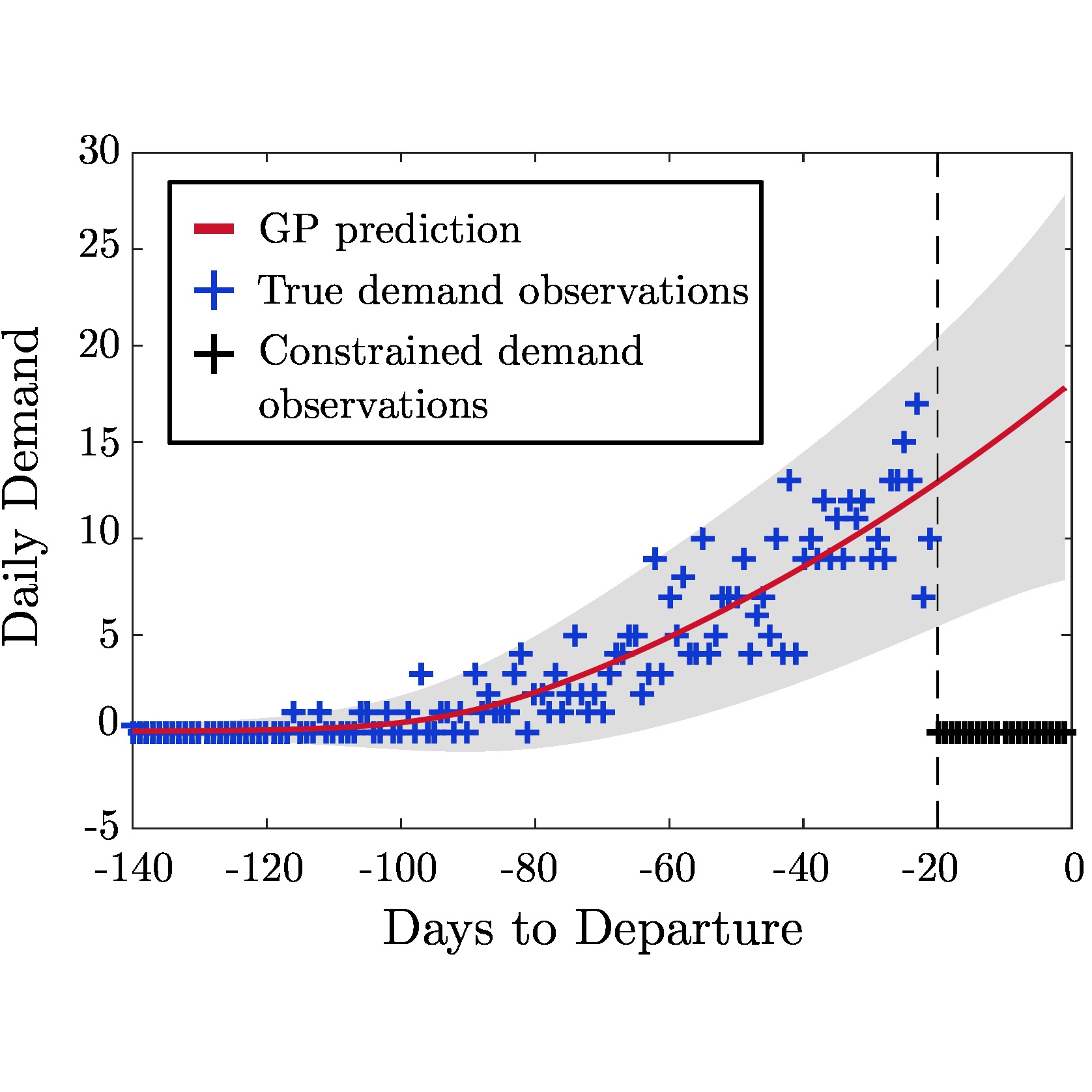
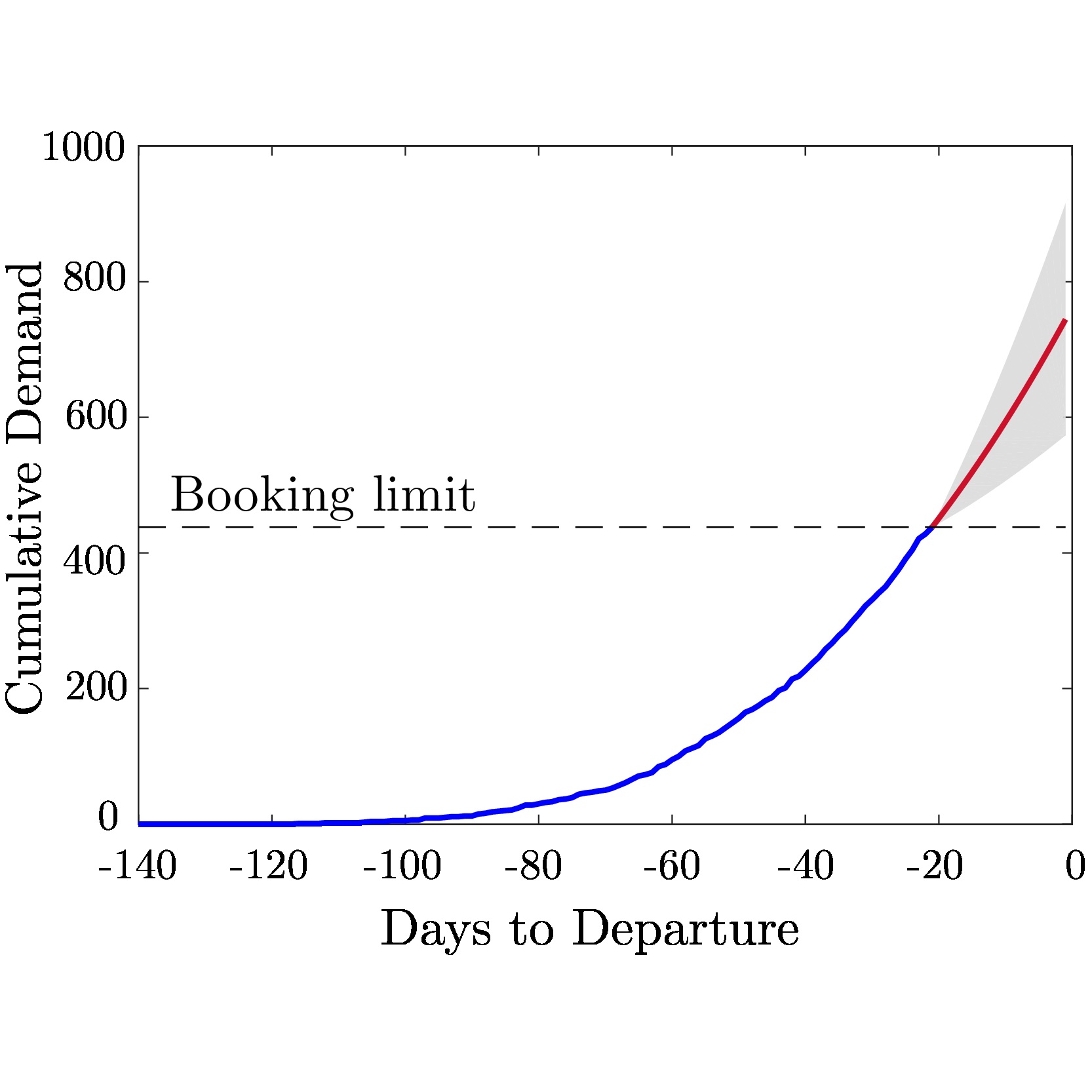
Figure 1: Illustration of GP regression for unconstraining demand. The figure on the left shows the mean prediction and confidence interval produced by our GP method, based on the true demand observations. The dotted black line indicates when the booking limit was reached, and the red line beyond this point shows the GP's unconstrained approximations. The figure on the right shows in red the reconstruction of the cumulative demand curve over the constrained period using the daily demand values predicted with the GP.
In the course of this inference procedure, we need to specify (i) a likelihood function or observation model, and (ii) a mean and covariance function for the GP prior.
Our model uses a Poisson likelihood, based on our implicit model of the bookings process as a doubly stochastic Poisson process, i.e. where bookings are determined by a Poisson process whose rate $\lambda$ is itself a Gaussian process (and thus changes over time).
For the GP prior, we use a zero mean function and define a new 'variable degree polynomial covariance function' \begin{equation} k(x,x') = \sigma^2(x^\top x' + c)^p, \end{equation} with $\theta_c = \{\sigma , c, p\}$ as the covariance hyperparameters (a modification of the polynomial covariance function in which $p$ is a fixed positive integer).
Having conducted a number of numerical experiments, our results are rather promising: the method compares favourably with state of the art methods when repeating experiments from recent literature. The added benefit, though, is that when these experiments are modified to have weaker assumptions on how the test data should look and be generated, our method maintains its strong performance better than its competitors. Our modifications included diversifying the shape of demand curve on which the methods were tested, as well as allowing for the presence of changepoints - points at which the characteristics of the underlying demand trend change dramatically. Using existing theory, we can elegantly extend our GP regression framework to cope with such situations by constructing an appropriate covariance function. For our purposes, we want to allow for the fact that the covariance before and after the changepoint might be completely different. We therefore redefine our covariance function to be \begin{align}\label{eq: Changepoint covariance} k(x,x') = \begin{cases} \sigma_1^2(x^\top x' + c_1)^{p_1} & \text{if } x,x' < x_c,\\ \sigma_2^2(x^\top x' + c_2)^{p_2} & \text{if } x,x' \geq x_c,\\ 0 & \text{otherwise}, \end{cases} \end{align} where $\theta = \{\sigma_1, \sigma_2, c_1, c_2, p_1, p_2, x_c\}$ are all hyperparameters inferred from the data. You can see an example of how well it performs in the image below."
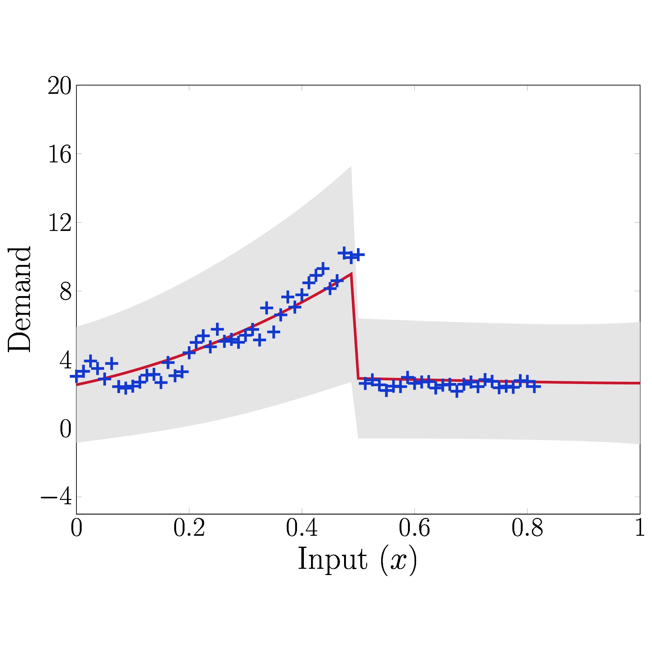
Figure 2: Illustration of automatic changepoint detection with GPs using our piecewise-defined variable degree polynomial covariance function.
You can read the research in greater detail here.