As part of our series of research articles deliberately focusing on the rigour and intricacies of mathematics and its problems, Oxford Mathematician David Seifert discusses his and his collaborator Catalin Badea's work.
Given a point $x$ and a shape $M$ in three-dimensional space, how might we find the point in $M$ which is closest to $x$? In general there need not be an easy answer, but suppose we have the extra information that $M$ is in fact the intersection of several sets which are much simpler to handle (so that a point lies in $M$ if and only if it lies in each of the simpler sets). In this case we might put the sets in order and proceed iteratively, by letting $x=x_0$ be the starting point in a sequence and taking $x_1$ to be the point closest to $x_0$ among the points in the first of the simpler sets. Next we find the point $x_2$ in the second simple subset which lies closest to $x_1$, and we continue in this way, returning to the first simple subset when we have exhausted the list. Does this process lead to the answer we want?
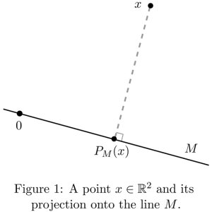
Recent research by Oxford Mathematician David Seifert and his collaborator Catalin Badea of Université de Lille 1 tackles this question not just in familiar three-dimensional space but in the much more general setting of Hilbert spaces. (Here and in what follows it is more the broad underlying ideas that matter, not so much the mathematical details.) Given a Hilbert space $X$ and a closed subspace $M$ of $X$, the orthogonal projection $P_M$ onto $M$ is the linear operator defined by the property that $P_M(x)$ is the point in $M$ which lies closest to $x\in X$. Figure 1 illustrates the case where $X$ is the Euclidean plane and $M$ is a line through the origin, but $X$ could also be a Sobolev space or some other infinite-dimensional Hilbert space. Many problems in mathematics, from linear algebra to the theory of PDEs, involve finding $P_M(x)$ for a given vector $x\in X$ and a space $M$. Sometimes $P_M(x)$ can be computed easily, but in other cases it cannot. Nevertheless, there is a natural way of finding an approximate solution if it is possible, as in the initial example, to break down our problem into easier subproblems.
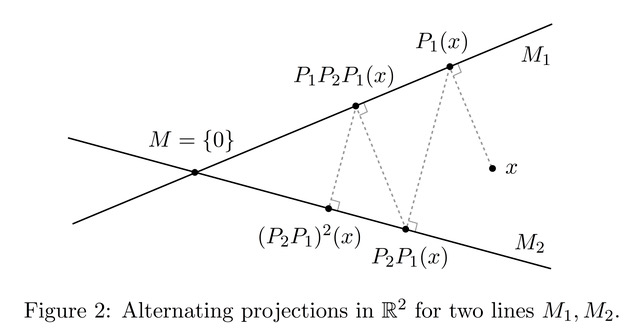
Indeed, suppose that $M=M_1\cap\dotsc\cap M_N$ where $M_1,\dots, M_N$ are themselves closed subspaces of $X$. We may not know much about $M$ or the operator $P_M$, but often the problem of finding the nearest point to a given vector $x\in X$ in any of the subspaces $M_k$, $1\le k\le N$, is much simpler. Writing $P_k$ for the orthogonal projection onto $M_k$, $1\le k\le N$, we may then successively find the vectors $P_1(x)$, $P_2P_1(x), \dots, P_N\cdots P_1(x)$, $P_1P_N\cdots P_1(x)$ and so on, projecting cyclically onto the subspaces $M_1,\dots,M_N$; see Figure 2.
This method of alternating projections has many different applications. These include surprising ones such as image restoration and computed tomography, but also linear algebra and the theory of PDEs. In linear algebra it corresponds to solving a system of linear equations one by one, at each stage finding the solution to the next equation which lies closest to the previous solution (the Kaczmarz method); in the theory of PDEs the method can capture the process of solving an elliptic PDE on a composite domain by solving it cyclically on each subdomain and using the boundary conditions to update the solution at each stage (the Schwarz alternating method). In general one is led to consider the single operator $T=P_N\cdots P_1$. It is known [2] that
$$ \|T^n(x)-P_M(x)\|\to0,\quad n\to\infty, \quad\quad\quad\quad(*) $$
for all $x\in X$, which means that by projecting cyclically onto the subspaces $M_1,\dotsc,M_N$ we may approximate the unknown solution $P_M(x)$ to arbitrary precision. In practice, though, this result is of limited value unless one has some knowledge of the rate at which the convergence takes place in $(*)$, so that one can estimate the number of iterations required to guarantee a specified level of precision. For example, in the Schwarz alternating method should we expect to require 50 iterations or 50,000 iterations in order to achieve a reasonably good approximation to the (unknown) true solution of our PDE?
There is a surprising dichotomy for the rate of convergence in $(*)$. Either the convergence is exponentially fast for all initial vectors $x\in X$, or one can make the convergence as slow as one likes by choosing appropriate initial vectors $x\in X$. In the example in Figure 2 the rate of convergence is determined by the angle between the lines $M_1$, $M_2$, and likewise in the general case the rate of convergence in $(*)$ depends in an interesting way on the geometric relationship between the subspaces $M_1,\dots,M_N$. In the case of the Schwarz alternating method, for instance, the crucial factor is the precise way in which the different subdomains overlap. If they overlap nicely then we will get exponentially fast convergence no matter where we start, and 50 iterations may well be enough to guarantee a good degree of approximation to the true solution. On the other hand, if the domains overlap in an unfavourable way then for certain starting points even 50,000 iterations may be insufficient. So is all lost if one is in the bad case of arbitrarily slow convergence?
Badea and Seifert showed in [1] that the answer is 'no'. More precisely they proved that even in the bad case there exists a dense subspace $X_0$ of $X$ such that for initial vectors $x\in X_0$ the rate of convergence in $(*)$ is faster than $n^{-k}$ for all $k\ge1$. This result provides a theoretical justification for a phenomenon observed by some practitioners, namely that even in bad cases one can usually achieve reasonably rapid convergence without having to experiment with too many different initial vectors $x\in X$. Badea and Seifert succeeded in improving the known results in other ways, too, for instance by giving a sharper estimate on the precise rate of convergence in the case where it is exponential. Underlying these results is the theory of (unconditional) Ritt operators. The theory of Ritt operators is closely related to some of David's earlier work [3, 4] on the quantified asymptotic behaviour of operators, and it is through this connection with operator theory that he first became interested in the method of alternating projections.
Is this the end of the story? As usual in mathematical research, answering one question opens up many more. In particular, Badea and Seifert's main result shows only that there is, in some sense, a rich supply of initial vectors leading to a decent rate of convergence in the method of alternating projections, but it does not say where these vectors should lie. This is an important open problem in approximation theory, and part of David Seifert's current research is concerned with developing techniques which can shed light on questions such as this.
References
- C. Badea and D. Seifert. Ritt operators and convergence in the method of alternating projections. J. Approx. Theory, 205:133–148, 2016.
- I. Halperin. The product of projection operators. Acta Sci. Math. (Szeged), 23:96–99, 1962.
- D. Seifert. A quantified Tauberian theorem for sequences. Studia Math., 227(2):183–192, 2015.
- D. Seifert. Rates of decay in the classical Katznelson-Tzafriri theorem. J. Anal. Math., 130(1):329–354, 2016