Christina Goldschmidt from the Department of Statistics in Oxford talks about her joint work with Louigi Addario-Berry (McGill), Nicolas Broutin (Paris Sorbonne University) and Gregory Miermont (ENS Lyon) on random minimum spanning trees.
"One of the most basic problems in combinatorial optimisation is the problem of finding the minimum spanning tree of a graph. We are given a connected graph $G = (V, E)$ whose edges are endowed with weights $(w_e, e \in E)$, where $w_e \ge 0$ for all $e \in E$. The weight of a subgraph of $G$ is the sum of the weights on its edges, and we seek a connected spanning subgraph of $G$ of minimal weight; it's easy to see that this must be a tree, called the minimum spanning tree (MST). (If the weights are all distinct then the MST is unique.) For example, we might think of the graph as representing a collection of cities and the edge-weights as representing the cost of building a road between its end-points; the MST is then the lowest-cost way of building a road-network which connects all of the cities.
The minimum spanning tree problem turns out to be easy to solve algorithmically, via one of several greedy algorithms. We will describe two of these algorithms, which are in some sense opposites. The first is known as Kruskal's algorithm, and proceeds as follows. List the edges as $e_1, e_2, \ldots$ in increasing order of weight (breaking ties arbitrarily), so that $w_{e_1} \le w_{e_2} \le \ldots$ We now construct the MST: go through the edges in the given order, and include an edge in the subgraph if and only if it does not create a cycle. The other algorithm (which we might call the reverse Kruskal algorithm, or the cycle-breaking algorithm) starts by listing the edges in decreasing order of weight, so that $w_{e_1} \ge w_{e_2} \ge \ldots$, and then goes through the edges one by one in this order, removing an edge if and only if it sits in a cycle. It's a nice exercise to check that these two procedures both yield the MST.
Let's now start with one of the simplest possible graphs: the complete graph on $n$ vertices (with vertices labelled from 1 to $n$), in which every possible edge between two vertices is present. What does a 'typical' MST of a large complete graph look like? In order to make sense of this question, we need a model. Let us assign the edges independent and identically distributed random weights, with uniform distribution on the interval $[0,1]$. (It doesn't actually matter which distribution we choose as long as it has the property that the probability of two edges having the same weight is 0, because the MST depends only on the induced ordering of the edges.) What can we say about the MST, $M_n$ given by this procedure, which is now a random tree with vertices labelled by 1 up to $n$? We're mostly going to be interested in asymptotics as $n \to \infty$.
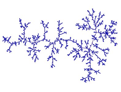
At first sight, you might think that the tree will just be uniform on the set of possibilities. Cayley's formula tells us that there are $n^{n-2}$ different trees on $n$ labelled vertices, and you might imagine that we are getting each of those with the same probability. This turns out to be very far from the truth! (Actually, you can check that they're not the same for, say, $n=4$, by a direct calculation). But we're mostly interested in what's happening for large $n$.) One way to characterise the difference is to ask how far apart two vertices typically are in these two trees. In the uniform random tree, $T_n$, if we pick two vertices uniformly at random, their distance apart is a random variable $D_n$ which is such that $n^{-1/2}D_n$ converges in distribution to a random variable $D$ as $n \to \infty$. So for a large instance of $T_n$, distances are typically varying in $n^{1/2}$. If you ask the same question in the MST, $M_n$, the answer turns out to be that typical distances vary in $n^{1/3}$.

Figure 1: A large uniform random tree
The best way to see this turns out to be via a connection with one of the most famous models from probabilistic combinatorics: the Erdős–Rényi random graph, $G(n,p)$. This is one of the simplest random graph models imaginable: take $n$ vertices, labelled from 1 to $n$, and for every possible edge include it with probability $p$ and don't include it otherwise, independently for different possible edges. It turns out that this model undergoes a so-called phase transition, a term we borrow from physics to mean a huge change in behaviour for a small change in some underlying parameter. Here, it turns out that the right parameterisation to take is $p = c/n$, where $c$ is a constant. For such a value of $p$, each vertex has a binomial number of neighbours with parameters $n-1$ and $c/n$, which has mean approximately $c$. Now, if $c < 1$, the graph contains only relatively small connected components, of size at most a constant multiple of $\log n$. On the other hand, if $c > 1$, the largest component occupies a positive proportion of the vertices, and all of the others are at most logarithmic in size. We refer to this phenomenon as the emergence of the giant component.
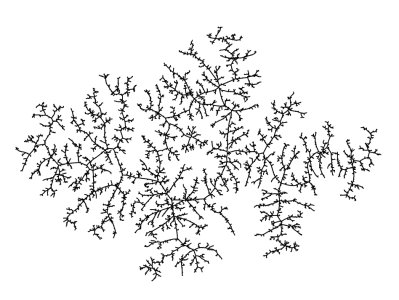
The behaviour is much more delicate at the point of the phase transition, $c = 1$. Here, there is an intermediate component size which appears: the largest components (and there are many of them!) have sizes on the order of $n^{2/3}$. In fact, this is true slightly more generally: we can take $p = 1/n + \lambda/n^{4/3}$ for any $\lambda \in \mathbb{R}$, and the same size-scaling occurs. This range of $p$-values is known as the critical window. For any point inside the critical window, if we let $C_1^n, C_2^n, \ldots$ be the sizes of the components, listed in decreasing order, then a beautiful result of David Aldous from 1997 says that $n^{-2/3} (C_1^n, C_2^n, \ldots)$ converges in distribution to a limit sequence $(C_1, C_2, \ldots)$ which is related to the lengths of the intervals of time which a Brownian motion with drift spends strictly above its running minimum. He also proved that the components are quite 'tree-like', in that each only has finitely many more edges than a tree on the same vertex-set. In joint work with Louigi Addario-Berry and Nicolas Broutin from 2012, I extended this result to give a full description of the limiting component structures. The right way to think about a limiting component is as a metric space: the vertices are the points of the metric space, and the distance between two vertices is the so-called graph distance, namely the number of edges traversed in the shortest path between them. Such a component has size on the order of $n^{2/3}$ (with a random pre-factor), so that in order to have any hope of getting a limit, we're going to need to rescale in some way. It turns out that we need to rescale the graph distance by $n^{-1/3}$ in order to get a nice limit metric space. The limiting components are sort of continuum analogues of tree-like connected graphs. (They're quite closely related to the limit of a large uniform random tree.)

Figure 2: A large component of a critical Erdős–Rényi random graph. Picture by Nicolas Broutin.
How does this help us to understand the MST? Firstly, let's introduce a particular way of building the Erdős–Rényi random graph $G(n,p)$. Start from the complete graph and use the same independent uniform edge-weights that we used to construct the MST, but now do something slightly different: simply keep every edge whose weight is less than or equal to $p$. Since a uniform random variable on $[0,1]$ is less than or equal to $p$ with probability $p$, this gives a realisation of $G(n,p)$. Moreover, we have a nice monotonicity in $p$, in that if we increase $p$, we include more edges. In other words, we can think of a process evolving in time, where 'time' is given by the value $p$, which varies from 0 to 1. Notice that this does something very similar to Kruskal's algorithm: as we increase $p$, every so often we reach the weight of the next edge on the list, it's just that in the Erdős–Rényi random graph setting we always include the edge, whereas in Kruskal's algorithm we only include it if it doesn't create a cycle. In particular, if we imagine doing both procedures simultaneously, then the difference between the two is that Kruskal's algorithm yields a forest at every step until its very final one when the subgraph becomes connected, whereas the Erdős–Rényi random graph process has more edges. But the vertex-sets of the components of the forest and graph are the same in the two cases: the only difference is edges which lie in cycles. If we take a snapshot of both processes at $p = 1/n + \lambda/n^{4/3}$ then the graph is still quite forest-like, in that each component only has a few more edges than the Kruskal forest.
What happens as we move through the critical window i.e. as we increase $\lambda$? The largest components gradually join together (they will eventually all be part of the giant) and we also insert more and more edges which create cycles. As we move through the critical window, whether a particularly vertex is contained in the current largest component is something that can be true for a bit and then cease to be true, or vice versa, as the components randomly aggregate. But if we take $\lambda$ to be large enough then eventually one component 'wins the race': its vertices remain within the largest component forever more. It turns out that the metric structure of the MST of this component is a good approximation to the metric structure of the MST of the whole graph: the difference between the two consists of a whole bunch of tiny trees which are glued on at points which are reasonably uniformly spread across the component, and thus don't make a huge difference to, for example, distances between typical vertices. There is a subtlety here, though: the vast majority of the vertices in the graph (an asymptotic proportion 1) are, at this point, still outside the largest component!
To get from the largest component of the Erdős–Rényi random graph process to its MST, we apply the cycle-breaking algorithm. We will only ever remove edges in cycles, so we can restrict our attention to the set $S$ of edges lying in cycles. If we just observe the component but not its edge-weights then the highest-weight edge lying in a cycle is simply uniformly distributed on $S$. Once we remove the highest-weight edge, we update $S$ to contain only the edges that still lie in cycles, and repeat the procedure of removing a uniform edge and updating until $S$ is empty. (Since we only have finitely many more edges than a tree, this procedure terminates.) This procedure turns out to pass nicely to the limit, and so we can make sense of the limiting MST of the largest component.
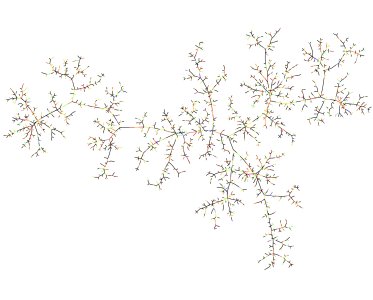
Making this argument rigorous takes quite a lot of work, but the upshot is we get the existence of a random compact metric tree-like space $M$ (the technical term is an $\mathbb{R}$-tree) such that if we rescale distances in $M_n$ by $n^{-1/3}$, we have convergence in distribution to $M$.
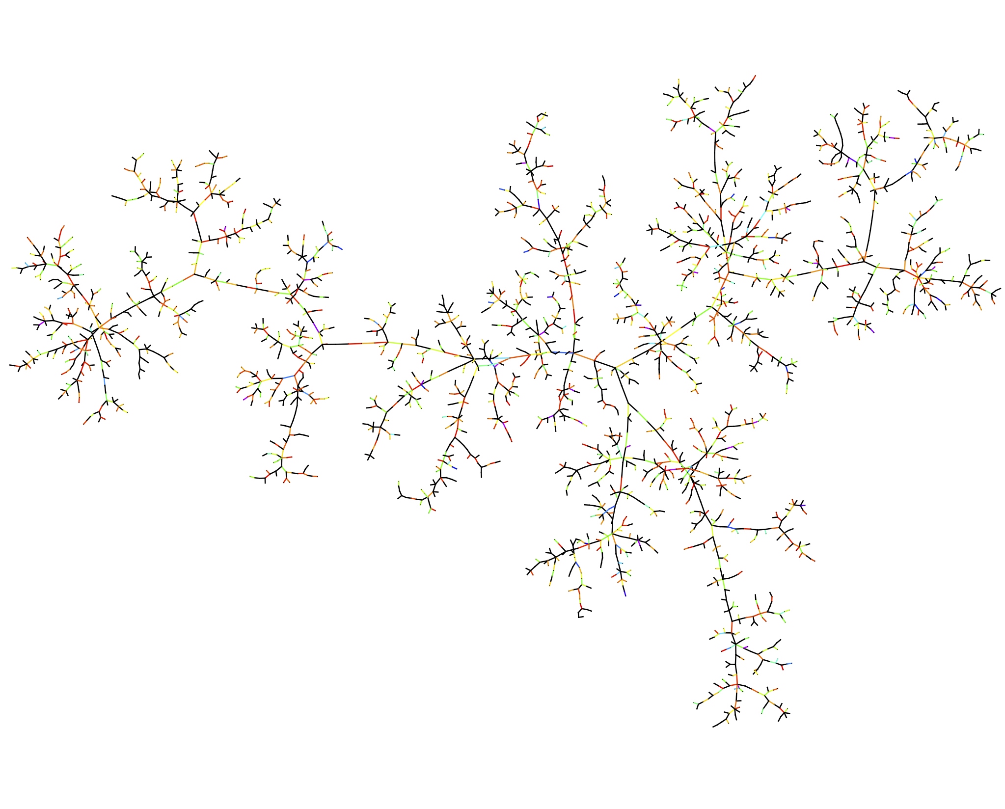
Figure 3: A realisation of the minimum spanning tree of the complete graph. Picture by Louigi Addario-Berry.
Lots of questions remain open about $M$. For example, in a uniform random tree $T_n$, we saw that the distance between two uniform points converges on rescaling by $n^{-1/2}$ to a limit $D$, which has an explicit distribution: we have $\mathbb{P}(D > x) = \exp(-x^2/2), x \ge 0$. This is just one aspect of a much more general result: the tree $T_n$, considered as a metric space with the graph distance rescaled by $n^{-1/2}$, converges in distribution to a limit $T$ which is known as the Brownian continuum random tree, and whose distributional properties are very well-understood. $D$ is the distance between two uniform points of $T$. The corresponding 'two-point distance' in $M$ is currently unknown. Understanding the distribution of this distance would be the first step in characterising the law of $M$. We do know some intriguing things about it, though. For example, $M$ is a random fractal, which turns out to be 3-dimensional: its Minkowski (or box-counting) dimension is 3 almost surely. This contrasts with $T$, which has Minkowski dimension 2 almost surely."
For more on this topic follow the links:
David Aldous, Brownian excursions, critical random graphs and the multiplicative coalescent, Annals of Probability 25, 2 (1997), pp.812-854.
Louigi Addario-Berry, Nicolas Broutin and Christina Goldschmidt, The continuum limit of critical random graphs, Probability Theory and Related Fields 152, 3-4 (2012), pp.367-406.
Louigi Addario-Berry, Nicolas Broutin, Christina Goldschmidt and Gregory Miermont, The scaling limit of the minimum spanning tree of the complete graph, Annals of Probability 45, 5 (2017), pp.3075-3144.