Oxford Mathematician Harald Oberhauser talks about some of his recent research that combines insights from stochastic analysis with machine learning:
"Consider the following scenario: as part of a medical trial a group of $2n$ patients wears a device that records the activity of their hearts - e.g. an electrocardiogram that continuously records the electrical activity of their hearts - for a given time period $[0,T]$. For simplicity, assume measurements are taken in continuous time, hence we get for each patient a continuous path $x=(x(t))_{t \in [0,T]}$, that is an element $x \in C([0,T],\mathbb{R})$, that shows their heart activity for any moment in the time period $[0,T]$. Additionally, the patients are broken up into two subgroups - $n$ patients that take medication and the remaining $n$ patients that form a placebo group that does not take medication. Can one determine a statistically significant difference in the heart activity patterns between these groups based on our measurements?
The above example can be seen as learning about the law of a stochastic process. A stochastic process is simply a random variable $X=(X_t)_{t \in [0,T]}$ that takes values in the space of paths $C([0,T],\mathbb{R})$ and the law $\mu$ of $X$ is a probability measure that assigns a probability to the possible observed paths. The above example amounts to drawing $n$ samples from a path-valued random variable $X$ with unknown law $\mu$ (the medicated group) and $n$ samples from a path-valued random variable $Y$ with unknown law $\nu$ (the placebo group). Our question about a difference between these groups amounts to asking whether $\mu\neq\nu$. Finally, note that this example was very simple, and in typical applications we measure much more than just one quantity over time. Hence, we discuss below the general case of $C([0,T],\mathbb{R}^e)$-valued random variables for any $e \ge 1$ ($e$ can be very large, e.g.~$e\approx 10^3$ appears in standard benchmark data sets).
But before we continue our discussion about path-valued random variables, let's recall the simpler problem of learning the law of a real-valued random variable. A fundamental result in probability is that if $X$ is a bounded, real-valued random variable, then the sequence of moments \begin{align} (1)\quad\label{moments} (\mathbb{E}[X], \mathbb{E}[X^2], \mathbb{E}[X^3], \ldots) \end{align} determines the law of $X$, that is the probability measure $\mu$ on $\mathbb{R}$ given as $\mu(A)= \mathbb{P}(X \in A)$. This allows us to learn about the law of $X$ from independent samples $X_1,\ldots,X_n$ from $X$, since \[\frac{1}{n}\sum_{i=1}^n X_i^m \rightarrow \mathbb{E}[X^m] \text{ as }n\rightarrow \infty\] for every $m\ge 1$ by the law of large numbers. This extends to vector-valued random variables, but the situation for path-valued random variables is more subtle. The good news is that stochastic analysis and a field called "rough path theory'' provides a replacement for monomials in the form of iterated integrals: the tensor \[ \int dX^{\otimes{m}}:= \int _{0 \le t_1\le \cdots \le t_m \le T} dX_{t_1} \otimes \cdots \otimes dX_{t_m} \in (\mathbb{R}^e)^{\otimes m} \] is the natural "monomial'' of order $m$ of the stochastic process $X$. In analogy to (1), we expect that the so-called "expected signature"' of $X$, \begin{align}(2)\quad\label{esig} (\mathbb{E}[\int dX], \mathbb{E}[\int dX^{\otimes{2}}], \mathbb{E}[\int dX^{\otimes 3}], \ldots) \end{align} can characterize the law of $X$. In recent work with Ilya Chevyrev we revisit this question and develop tools that turn such theoretical insights into methods that can answer more applied questions as they arise in statistics and machine learning. As it turns out, the law of the stochastic process $X$ is (essentially) always characterized by (2) after a normalization of tensors that ensures boundedness of this sequence. Mathematically, this requires us to understand phenomena related to the non-compactness of $C([0,1],\mathbb{R}^d)$. Inspired by results in machine learning, we then introduce a metric for laws of stochastic processes, a so-called "maximum mean discrepancy'' \begin{align} d(\mu,\nu)= \sup_{f} |\mathbb{E}[f(X)] - \mathbb{E}[f(Y)]| \end{align} where $\mu$ denotes the law of $X$ and $\nu$ the law of $Y$ and the $\sup$ over a sufficently large class of real-valued functions $f:C([0,T], \mathbb{R}^e) \rightarrow \mathbb{R}$. To compute $d(\mu,\nu)$ we make use of a classic "kernel trick'' that shows that \begin{align} (3) \quad\label{mmd} d(\mu,\nu) = \mathbb{E}[k(X,X')] - 2\mathbb{E}[k(X,Y)] + \mathbb{E}[k(Y,Y')] \end{align} where $X'$ resp.~$Y'$ are independent copies of $X\sim\mu$ resp.~$Y\sim \nu$ and the kernel $k$ is the inner product of the sequences of iterated integrals formed from $X$ and $Y$. Previous work provides algorithms that can very efficiently evaluate $k$. Combined with (3) and the characterization of the law by (2), this allows us to estimate the metric $d(\mu,\nu)$ from finitely many samples.
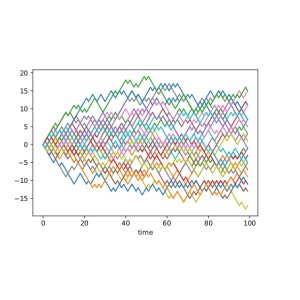
An immediate application is a two-sample test: we can test the null hypothesis \[ H_0: \mu=\nu \text{ against the alternative }H_1: \mu\ne \nu \] by estimating $d(\mu,\nu)$ and rejecting $H_0$ if this estimate is bigger than a given threshold. Recall our example of two patient groups (medicated and placebo). The question whether there's a statistical difference between these groups can be formalized as such a two-sample hypothesis test. To gain more insight it can be useful to work with synthetic data (after all, the answer to a two-sample test will be a simple yes or no depending on whether to reject the null hypothesis). Therefore consider the following toy example: $\mu$ is the law of a simple random walk and $\nu$ is the law of a path-dependent random walk; Figure 1 shows how samples from these two stochastic processes look; more interestingly Figure 2 shows the histogram of an estimator for $d(\mu,\nu)$. We see that the support is nearly completely disjoint which indicates that the test will perform well and this can be made rigorous and quantitative.
These examples of $e=1$-dimensional paths are overly simplistic - we can already see a difference by looking at the sampled paths. However, this situation changes drastically in the higher-dimensional setting of real-world data; some coordinates might evolve quickly, some slowly, others might not be relevant at all, often the statistically significant differences are in the complex interactions between some coordinates; all subject to noise and variations. Finally, the index $t \in [0,T]$ might not necessarily be time; for example, in a recent paper with Ilya Chevyrev and Vidit Nanda (featured in a previous case-study), the index $t$ is the radius of spheres grown around points in space and the path value for every $t>0$ is determined by a so-called barcode from topological data analysis that captures the topological properties of these spheres of radius $t$"

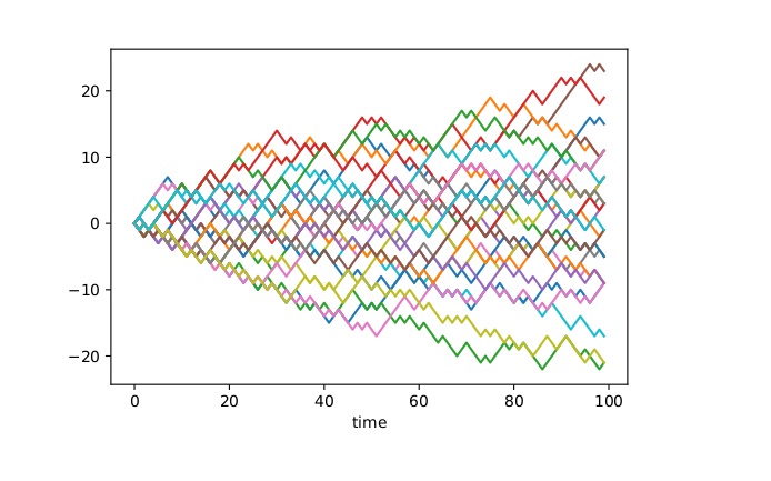
Figure 1: The left plot shows 30 independent samples from a simple random walk; the right plot shows 30 independent samples from a path-dependent random walk.
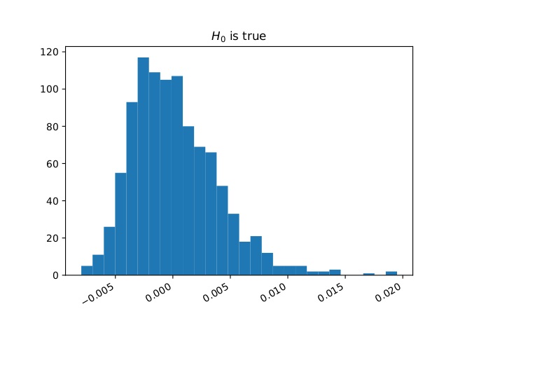
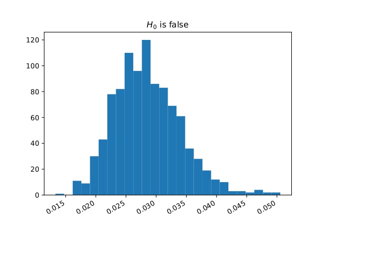
Figure 2: The left plot shows the histogram for an estimator of $d(\mu,\nu)$ if the null hypothesis is true, $\mu=\nu$ (both are simple random walks); the right plot shows the same if the null is false ($\mu$ is a simple random walk and $\nu$ is a path-dependent random walk as shown in Figure 1.