Oxford Mathematicians Andy Allan and Sam Cohen talk about their recent work on estimating with uncertainty.
"In many examples, we need to use indirect observations to estimate the state of an unseen object. A classic example of this comes from the Apollo missions: how could the crew use observations of the relative position of the sun, moon and earth to determine their position and velocity, and so correct their trajectory? The same ideas have been used in many problems since, from speech recognition to animal tracking to estimating the risk in financial markets. The problem of estimating the current state of such a hidden process from noisy observations is known as stochastic filtering.
To solve this problem, we often begin by assuming that we know 1) how the unseen quantity (the spacecraft's position and velocity) is changing and 2) how our observations relate to the unseen quantity. Both of these can have random errors, but we assume we know what the errors 'typically' look like. For a rocket, these are well understood, but in other applications, we may only have a rough estimate of how these should be modelled, and want to take that uncertainty into account in our calculations.
In our recent work, we investigate how to do this estimation in a way which is robust to errors in our model - instead of directly estimating the hidden state, we first calculate how 'reasonable' each possible model is, then try to ensure our estimates work well for all reasonable models. This is difficult, as random observations make our problem too 'rough' for the usual mathematical approaches to work.
In order to give a more precise description of the problem, suppose that we are interested in the position of some 'signal' process $S$, but we are only able to observe some separate 'observation' process $Y$. A classic example is when $S$ and $Y$ satsify the linear equations \begin{align*} d S_t &= (\theta_t + \alpha S_t)\,d t + \sigma\,d B^1_t,\\ d Y_t &= cS_t\,d t + d B^2_t, \end{align*} where $\theta, \alpha, \sigma$ and $c$ are various (in general time-dependent) parameters, and $B^1, B^2$ are some random noise (which we assume to be independent Brownian motions).
Let us write $\mathcal{Y}_t$ for our observations of $Y$ up to time $t$. In this setting the posterior distribution of the signal $S_t$ at time $t$, given our observations $\mathcal{Y}_t$, can be shown to be Gaussian, i.e. $S_t|\mathcal{Y}_t \sim N(x_t,V_t)$. Moreover, the conditional mean $x_t = \mathbb{E}[S_t\,|\,\mathcal{Y}_t]$ and variance $V_t = \mathbb{E}[(S_t - x_t)^2\,|\,\mathcal{Y}_t]$ satisfy the Kalman-Bucy filtering equations: \begin{align*} d x_t &= (\theta_t + \alpha x_t)\,d t + cV_t(d Y_t - cx_t\,d t),\\ \frac{d V_t}{d t} &= \sigma^2 + 2\alpha V_t - c^2V_t^2. \end{align*}
This works provided that we know the exact values of all the parameters of the model. However, let us now suppose for instance that the parameter $\theta$ in the above is unknown, or we are worried that it may have been miscalibrated. It might also be the case that $\theta$ itself varies through time, but we are unsure of its dynamics. In either case, this means that there is uncertainty in the dynamics of the posterior mean $x_t$.
At a given time $t$, we are therefore uncertain of the 'true' posterior distribution of $S_t$. However, we know that it must be a Gaussian distribution with some mean $x_t = \mu \in \mathbb{R}$. What we would like to know is, given our observations, how 'reasonable' is each choice of posterior mean $\mu$?
Given a fixed $\mu \in \mathbb{R}$, there are infinitely many different choices of the parameter $\theta$ (each with a corresponding initial value $x_0$) which would have resulted in the terminal value $x_t = \mu$ for the posterior mean. That is, for each parameter choice $\theta \colon [0,t] \to \mathbb{R}$ we obtain a trajectory $x^\theta \colon [0,t] \to \mathbb{R}$ satisfying the filtering equation with parameter $\theta$, and the terminal condition $x^\theta_t = \mu$.
We can then consider penalising each such trajectory $x^\theta$ according to how 'unreasonable' we consider it to be. For example, if we believe the 'true' parameter $\theta$ should be fairly close to some specified value, then the severity of the penalisation for a particular $\theta$ can depend on how far it strays from this value. Moreover, we can consider penalising trajectories according to the likelihood of our observations under each parameter.
For a given posterior mean $\mu$, we then wish to find the most 'reasonable' trajectory, i.e. the one with the least associated penalty. In other words, we wish to minimise a 'cost functional' subject to a constraint: an optimal control problem. Although we are in a stochastic setting, the optimisation here should be performed separately for each possible realisation of the observation process. (There is no point averaging over all possible realisations of the observation process when it has already been observed!) This is therefore an instance of pathwise stochastic optimal control, and thus in general requires a pathwise approach to stochastic calculus (rough path theory).
The value function of this control problem characterises how reasonable we consider different choices of the posterior mean $x_t = \mu$ and the unknown parameter $\theta_t$ to be. In particular, the minimum point of this function tells us the 'most reasonable' mean $\mu$ and parameter value $\theta_t$. We establish this function as the unique solution of a (rough) Hamilton-Jacobi equation.
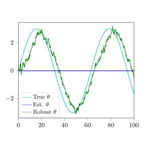
We illustrate our results with a numerical example. Here we take $\alpha = -0.3$, $\sigma = 0.5$ and $c = 1$. We suppose the (unknown) true parameter $\theta$ is a sine function, but that our best estimate of $\theta$ is the constant value $0$ (i.e. the long-time average of the true $\theta$); see Figure 1. We then simulate a realisation of the signal and observation processes.
Solving the Hamilton-Jacobi equation driven by this simulated observation path and evaluating the minimum point of the solution (i.e. the value function of our control problem), we obtain robust estimates of $S_t$ and $\theta_t$. In Figure 1 we plot the most reasonable value of the parameter $\theta_t$, given our observations, and compare it with the true and estimated parameter values.
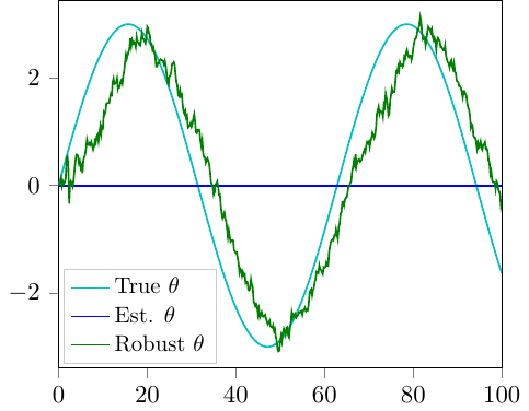
Figure 1: Learning θ.
In particular, the solution is able to 'learn' the true parameter value $\theta_t$ without assuming precise knowledge of the dynamics of $\theta$, we just assume that it's 'not too far from zero'.
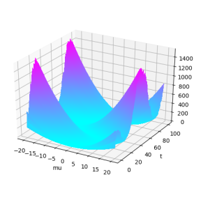
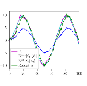
In Figure 2 we plot the $\mu$-component of the value function, and see how this function evolves in time. The minimum point of this function, i.e. the most reasonable value of the posterior mean $\mu$, is then shown in Figure 3. We also compare this 'robust filter' to the signal $S_t$ itself, as well as the standard Kalman-Bucy filter $x_t = \mathbb{E}[S_t\,|\,\mathcal{Y}_t]$, calculated using both the true and 'estimated' parameters.
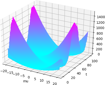
Figure 2: ‘Unreasonableness’ of each possible posterior mean µ.
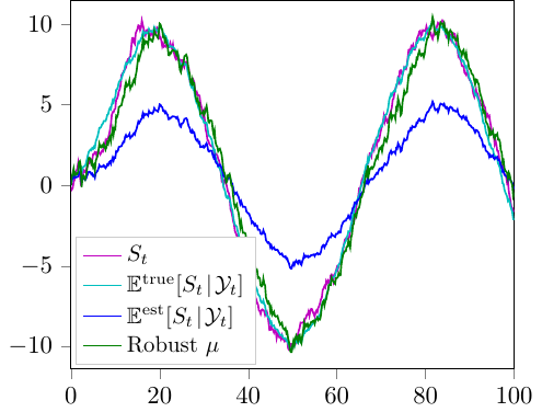
Figure 3: Estimates of St.
For all the details on this approach see:
A.L. Allan and S.N. Cohen, Parameter Uncertainty in the Kalman-Bucy Filter
A.L. Allan and S.N. Cohen, Pathwise Stochastic Control with Applications to Robust Filtering