Applied mathematics provides a collection of methods to allow scientists and engineers to make the most of experimental data, in order to answer their scientific questions and make predictions. The key link between experiments, understanding, and predictions is a mathematical model: you can find many examples in our case-studies. Experimental data can be used to calibrate a model by inferring the parameters of a real-world system from its observed behaviour. The calibrated model then enables scientists to make quantifiable predictions and quantify the uncertainty in those predictions.
There are two important caveats. The first is that, for any one scientific phenomenon, there can be as many models as there are scientists (or, probably, more). So, which should you choose? The second is that “all models are wrong, but some are useful". Often, those that include a high level of detail, and have the potential to make accurate quantitative predictions, are far too complicated to efficiently simulate, or for mathematicians to analyse. On the other hand, simple models are often amenable to analysis, but may not include all the important mechanisms and so cannot make accurate predictions. So how does one go from experimental observations to an understanding of the underlying science, when many different models of variable accuracy and tractability are available to reason with?
In a forthcoming paper, accepted for publication in the SIAM/ASA Journal of Uncertainty Quantification, Oxford Mathematicians Thomas Prescott and Ruth Baker have presented a multifidelity approach to model calibration. The model calibration procedure often requires a very large number of model simulations to ensure that the parameter estimate is reliable (i.e. has a low variance). Due to the large number of simulations required, it may not be feasible to calibrate the accurate model within a reasonable timeframe. Suppose there exists a second model which is much quicker to simulate, but inaccurate. The increased simulation speed means that it is more practical to calibrate this second model to the data. However, although the inaccurate model can be calibrated more quickly, its inaccuracy means that the resulting estimate of the system’s parameters is likely to be biased (see Fig. 1).
The model calibration task aims to achieve an unbiased estimate of the model’s parameters that balances between two conflicting aims: ensuring that the resulting estimates have reasonably small variance, but also that they are produced in a reasonably quick time. By combining each model’s strengths (the short simulation time of one, and the accuracy of the other), the key result of this project deals with the following question: how can the inaccurate model be used to calibrate the accurate model? In particular, how much simulation time should be given to simulating each of the models, and how should those simulations be combined? The result is a model calibration algorithm, tuned according to a formula that determines how to optimally share the computation effort between the two models. This algorithm enables the accurate model to be calibrated with an unbiased parameter estimate and with a significantly improved trade-off between variance and speed.
The results can be applied to speed up the calibration of many types of complicated mathematical models against experimental data, whenever a simpler alternative model can be used to help. These applications exist in fields as varied as ecology, physiology, biochemistry, genetics, engineering, physics, and mathematical finance.
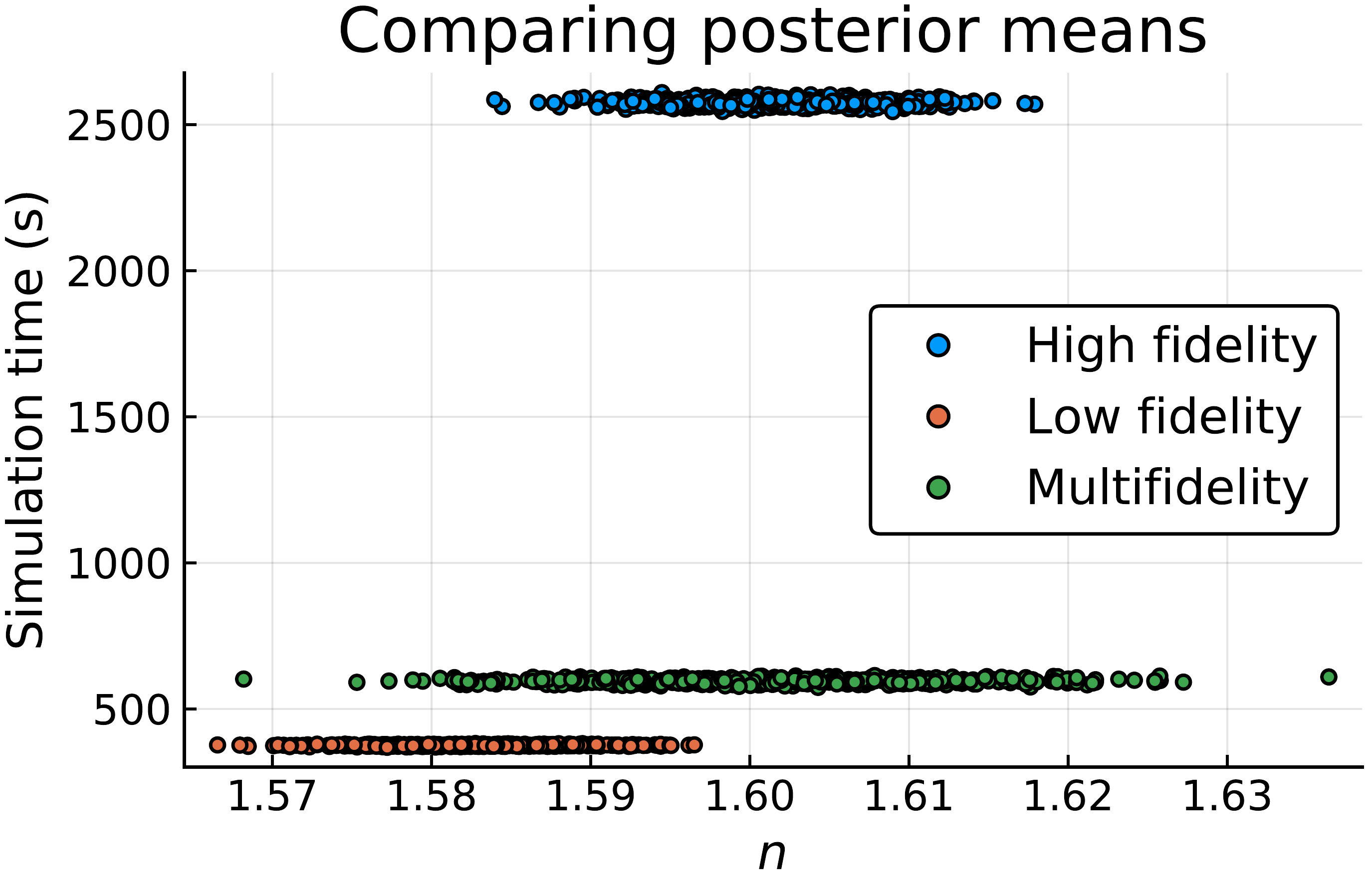
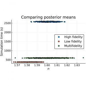
Fig 1. In blue are 500 estimates of a parameter n, each of which was generated using 10,000 simulations of a slow, accurate model, and taking around 40 minutes each. In orange are 500 estimates that each took only around 7 minutes to generate by simulating a fast, inaccurate model instead. These estimates are biased (i.e. centred around the wrong value). The estimates in green are where, for every 10 simulations of the inaccurate model, we also produced one simulation of the accurate model. This allows us to remove the bias. But here we see the effect of the trade-off: while the total simulation time is greatly reduced relative to the accurate model (to 10 minutes), this is at the cost of an increased variance (i.e. spread) of the estimate.