
Oxford Mathematicians Dmitry Belyaev and Michael McAuley explain the ubiquitous role of Gaussian Fields in modelling spatial phenomena across science, and especially in cosmology. This case-study is based on work with Stephen Muirhead at Queen Mary University of London (QMUL).
Smooth Gaussian fields are a type of random mathematical object, which are used throughout the sciences for modelling spatial phenomena. As an example, imagine looking at a region of the ocean fixed at some moment in time. The surface of the water, which will be random due to currents and waves, can be thought of as a Gaussian field.
Gaussian fields are particularly important in the study of cosmology. The Cosmic Microwave Background is weak electromagnetic radiation which can be detected from any point in space. This is a remnant of the extremely intense radiation emitted during the Big Bang, and can therefore be used to study the early universe. The intensity of this radiation depends on the direction it comes from, and so can be thought of as random. Cosmological theories predict that observations of this radiation on Earth can be modelled as a Gaussian field. So the intensity of the radiation at each point on Earth is analogous to the height of the ocean at each point in the previous example (see Figure 1 above). Studying the properties of Gaussian fields mathematically, can therefore help in developing and testing cosmological theories.
(Figure 1 above: an observation of the Cosmic Microwave Background. Red regions have higher intensity of radiation. Source: Planck 2018).
There are many other applications of Gaussian fields, in subjects as diverse as medical imaging, quantum mechanics and machine learning. One of the beautiful aspects of mathematics, is that we can simultaneously study all of these very different situations through abstraction.
One interesting property of Gaussian fields, is the number of regions where it exceeds a certain value, which can be thought of as the number of `hotspots' (on Figure 1 this would be the number of red regions). This has some particular applications in testing cosmological theories.
Many geometric properties of Gaussian fields are said to be `local', which means that they can be studied by breaking the domain into tiny pieces and adding up the result. For example, the total area of all hotspots is local, because it can be found by adding up the area of hotspots contained in each piece of the domain. Local quantities can be understood very well using a tool known as the Kac-Rice formula. The number of hotspots, however, is non-local, because when looking at two tiny pieces of the domain, we do not know whether the red regions in those two pieces are connected. This makes the number of hotspots difficult to study mathematically, as one must account for interactions between different regions of the Gaussian field.
In the last five years, it has been shown that for stationary Gaussian fields (i.e. those which are statistically the same at every point) the average number of hotspots is proportional to the area of the domain. So when looking at a Gausssian field on a large square of area $R^2$, the average number of hotspots is proportional to $R^2$.
The natural next step in understanding the number of hotspots is to study its variance, which is a non-negative number describing how much this quantity typically differs from its average due to randomness. Physicists have used non-rigorous methods to predict that, for a stationary Gaussian field, the variance of the number of hotspots in a square of area $R^2$ should be proportional to $R^2$.
Our work confirms half of this prediction: we show that for many stationary Gaussian fields, the variance is at least of order $R^2$. This bound is believed to be optimal for general fields. We also show that for one special field (see Figure 2), which has applications in quantum mechanics, the physics prediction is incorrect: the variance of the number of hotspots in a square of area $R^2$ is at least of order $R^3$.
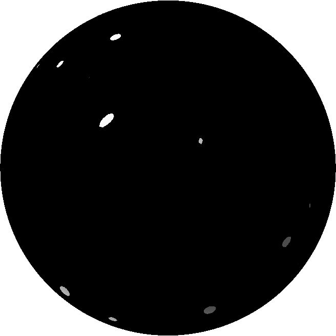
Figure 2: the hotspots of a particular Gaussian field above a given intensity are shown in black. This intensity increases throughout the animation, so that the hotspots shrink.