Oxford Mathematician Patrick Kidger writes about combining the mathematics of differential equations with the machine learning of neural networks to produce cutting-edge models for time series.
What is a neural differential equation?
Differential equations and neural networks are two dominant modelling paradigms, ubiquitous throughout science and technology respectively. Differential equations have been used for centuries to model widespread phenomena from the motion of a pendulum to the spread of a disease through a population. Meanwhile, over the past decade, neural networks have swept the globe as a means of tackling diverse tasks such as image recognition and natural language processing.
Interest has recently focused on combining these into a hybrid approach, dubbed neural differential equations. These embed a neural network as the vector field (the right hand side) of a differential equation - and then possibly embed that differential equation inside a larger neural network! For example, we may consider the initial value problem
$z(0) = z_0, \qquad \frac{\mathrm{d}z}{\mathrm{d}t}(t) = f_\theta(t, z(t))$
where $z_0$ is some input or observation, and $f_\theta$ is a neural network, and the output of the model may for example be taken to be $z(T)$ for some $T > 0$.
This is called a neural ordinary differential equation. At first glance one may be forgiven for believing this is an awkward hybridisation: a chimera of two very different approaches. It is not so!
Fitting parameterised differential equations to data has long been a cornerstone of mathematical modelling. The only difference now is that the parameterisation of the right hand side (the $f_\theta$) is a neural network learnt from data, rather than a theoretical one...derived from data (via the human designing it).
Meanwhile, it turns out that many standard neural networks may actually be interpreted as approximations to neural differential equations: in fact it seems that it is actually because of this that many neural networks work as well as they do. (Those doing traditional differential equation modelling are unsurprised. They've been using differential equations all this time precisely because they're such good models.)
Neural differential equations have applications to both deep learning and traditional mathematical modelling. They offer memory efficiency, the ability to handle irregular data, strong priors on model space, high capacity function approximation, and draw on a deep well of theory on both sides.
Neural controlled differential equations
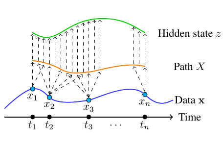
Against this backdrop, we consider the specific problem of modelling functions of time series. For example, we might observe a sequence of observations representing the vital signs of a patient in a hospital (heart rate, laboratory measurements, and so on). Is the patient healthy or not? We would like to build a model that determines this automatically. (Perhaps to automatically and rapidly alert a doctor if something seems amiss.)
Of course, there's a few ways of accomplishing this. In line with the theme of this article, the one we're going to introduce is a model of the following form:
$\mathrm{d}z(t) = f_\theta(t, z(t)) \,\mathrm{d}X(t)$
This is a neural controlled differential equation. If we had a "$\mathrm{d}t$" on the right hand side, instead of the "$\mathrm{d}X(t)$", then this would just be the neural ordinary differential equation we saw above. Having a "$\mathrm{d}X(t)$" instead means that the differential equation can change in response to the input $X$, which is a continuous-time path representing how the observations (of heart rate etc.) change over time.
If you're not familiar with this notation, then just pretend you can "divide by $\mathrm{d}t$" (or $\mathrm{d}X(t)$) and you get the equation we had earlier. Check out the paper [1] for a less hand-wavy explanation of what's really going on here.
Changes in $X$ will create changes in $z$. By training this model (picking a good $f_\theta$), we can arrange it so that if something happens in $X$ - for example a patient's health starts deteriorating - then we can produce a desired change in $z$ - which can be used to call a doctor.
Neural controlled differential equations are actually the continuous-time limit of recurrent neural networks. (Which would often be the typical way to approach this problem.) By pushing to the continuous-time limit we can get improved memory efficiency, can more easily handle irregular data... and also produce something theoretically beautiful! In keeping with what we argued earlier, it seems that recurrent neural networks often work because they look like neural controlled differential equations. Indeed the two most popular types of recurrent neural networks - GRUs and LSTMs - are explicitly designed to have features that make them look like differential equations. Not a coincidence! Understanding these relations will help us build better and better models as we go into the future.
Further reading:
This has been a short introduction to the nascent, fascinating field of neural differential equations. If you'd like to find out more about neural controlled differential equations, then check out [1]. For an idea of some of the things you can do with neural differential equations (like generating pictures, or modelling physics), then [2] has some nice examples. And for the paper that kickstarted the field in its modern form, check out [3].
[1] Kidger, Morrill, Foster, Lyons, Neural Controlled Differential Equations for Irregular Time Series, Neural Information Processing Systems 2020
[2] Kidger, Chen, Lyons, "Hey, that's not an ODE": Faster ODE Adjoints with 12 Lines of Code, arXiv 2021
[3] Chen, Rubanova, Bettencourt, Duvenaud, Neural Ordinary Differential Equations, Neural Information Processing Systems 2018