What takes a mathematician to the Arctic? In short, context. The ice of the Arctic Ocean has been a rich source of mathematical problems since the late 19$^{th}$ century, when Josef Stefan, aided by data from expeditions that went in search of the Northwest Passage, developed the classical Stefan problem. This describes the evolution of a moving boundary at which a material undergoes a phase change. In recent years, interest in the Arctic has only increased, due to the rapid changes occurring there due to climate change. The Arctic is particularly sensitive to changes in global temperatures, with consequences for the rest of the northern hemisphere that can include extreme weather events such as the 'Beast from the East' event in 2018.
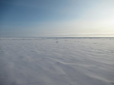
In 2019, I, Oxford Mathematician Michael Coughlan, undertook fieldwork as part of the SODA project in the central Arctic aboard the USCGC Healy (with Martin Doble of Polar Scientific Ltd.), deploying buoys onto the ice between $70^{\circ}$ and $80^{\circ}$N, that would drift with the currents and measure conditions above, below and within the ice. While there, I also took measurements of the ice floes on which we were working, and made observations of the ice and the ocean to inform my modelling work.
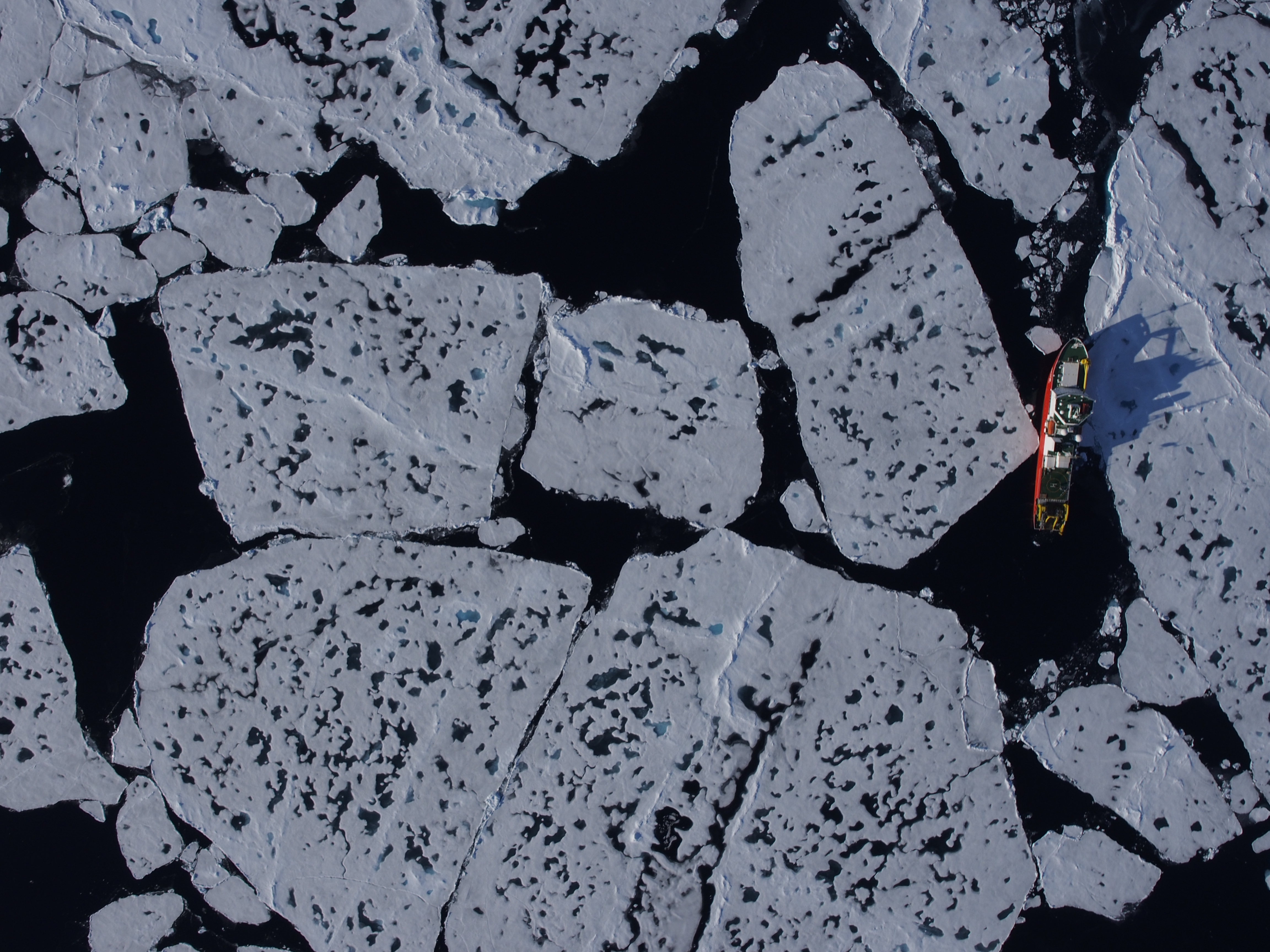
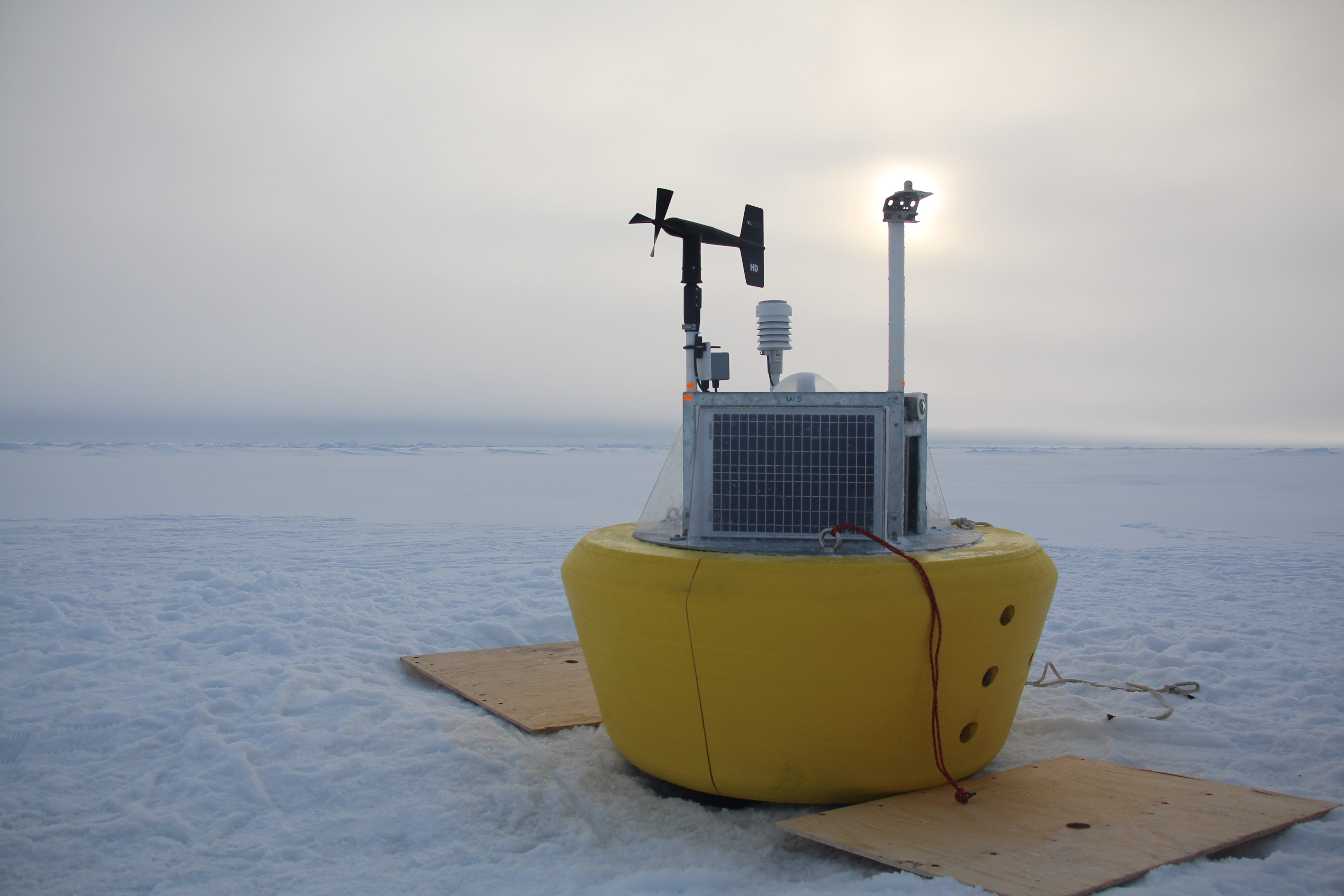
Figure 1: Melt ponds in Arctic Ocean, 2014. Pictured is the icebreaker RV Araon, which (for scale) is $110$m long. Photo: M. Doble. Polar Scientific Ltd. (b) Buoy deployment, Beaufort Sea, September 2019.
My work - with Oxford Mathematicians Ian Hewitt, Sam Howison, and Oxford Physicist Andrew Wells - focusses on modelling the formation and evolution of melt ponds on sea ice - features that form when water from the melting surface of the ice settles in the hollows and troughs of the topography. These can contribute further to melting of the floes, as water absorbs much more light than the surrounding ice, a phenomenon known as the ice-albedo feedback. The presence of surface water thereby hastens melting of the ice below it, often leading to the fracturing and break-up of floes (Arntsen et al., 2015). Due to the feedback effect, care must be taken to incorporate the behaviour of ponds in climate models, and my research investigates how to do this.
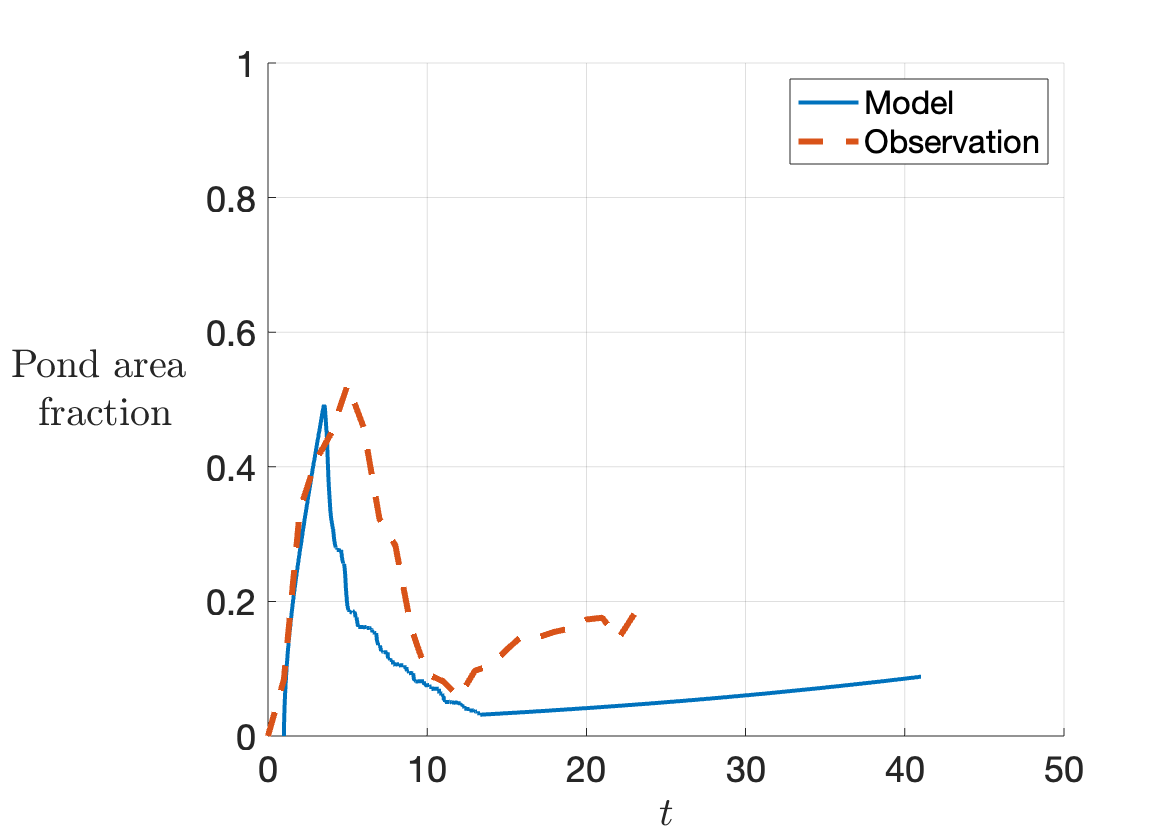
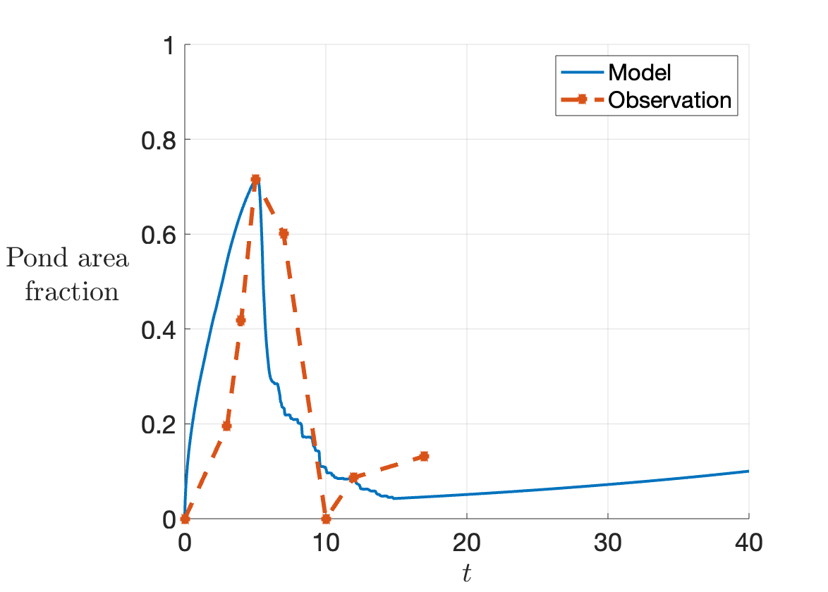
Figure 2: Time series of modelled area fraction of ponds (pond area as a fraction of total floe area) compared to data from two field experiments by Polashenski et al (2012). Time is measured from the onset of ponding. Left: 'North' site. Right: 'South' site.
Ponds display a range of geometries, from simple, single ponds, with areas of the order of several square metres, to large clusters, made up of what were previously many individual ponds, which can span areas of many hundreds of square metres (Hohenegger et al., 2012). These geometries are due in part to the distinct life cycle of ponds, which form initially where water from bare ice flows to the lowest parts of individual catchments in the topography. They then grow, begin to join one another and can eventually flood the whole floe. Interestingly, however, once the ice warms enough, it becomes permeable and the ponds drain into the sea. From then on, ponds only remain where the ice surface lies below sea level. Ponds also melt and sculpt the ice underneath them. Therefore, the history of their growth has an effect on their geometry and extent once the ponds drain to sea level.
We model the growth and evolution of ponds on a network in which the nodes are individual catchments, and links exist between each pair of nodes that neighbour one another. We express the behaviour of the ponds as a dynamical system on a network.
To do so we assign a dynamical variable which we call the activity, $x_i(t)$, to each node. A dynamical system can be written on the network as \begin{equation}\label{eq:activity} \dot{x_i} = f_i(x_i,t) + A_{ij}g_{ij}(x_i,x_j,t), \end{equation} where $f$ is a function of the node attributes and activity and $g$ represents how neighbouring nodes affect each other (Porter and Gleeson, 2016). The adjacency matrix $A_{ij}$ encodes the network structure. Here, the activity is the pond water level in each catchment. The function $f$ represents the contribution of melt-water both inflowing from the bare ice in the catchment, and the ice melting at the pond floor, derived from parametrised melt rates for bare and pond-covered ice, and conservation of mass. The function $g$ represents the fluxes between neighbouring catchments, which can take the form of one pond overflowing into another or two ponds joining together. Drainage is incorporated with the addition of a special 'ocean' node connected to each catchment, and a possible flux through the ice along each of the corresponding links.
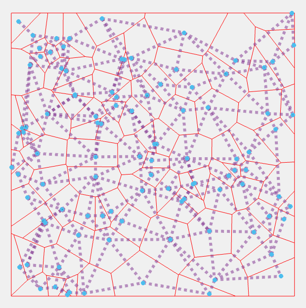
Figure 3: Visualisation of pond geometry and network structure for an ice floe. Dotted lines denote inactive edges, solid blue denote joins, and dashed yellow lines denote overflows. Greyed areas denote ponded regions. Red lines denote the boundaries between catchments. Blue circles denote draining catchments.
Time series of pond area predicted by the model are shown in Figure 2, compared to field data (Polashenski et al, 2012). The model shows good qualitative agreement with data, and resolves the important features of the life cycle of ponds. The model can be used to estimate the duration of the different processes in the life cycle, and affords us a computationally cheap way to parametrize pond dynamics. Further, by varying the parameters, we can explore how pond extent is likely to change as the Arctic warms.
Bibliography:
A. E. Arntsen, A. J. Song, D. K. Perovich, and J. A. Richter-Menge. Observations of the summer breakup of an Arctic sea ice cover. Geophys. Res. Lett., 42(19): 8057–8063, 2015. ISSN 19448007. doi: 10.1002/2015GL065224.
C. Hohenegger, B. Alali, K. R. Steffen, D. K. Perovich, and K. M. Golden. Transition in the fractal geometry of Arctic melt ponds. Cryosph., 6(5):1157–1162, 2012. ISSN 19940416. doi: 10.5194/tc-6-1157-2012.
C. Polashenski, D. Perovich, and Z. Courville. The mechanisms of sea ice melt pond formation and evolution. J. Geophys. Res. Ocean., 117(1):1–23, 2012. ISSN 21699291. doi: 10.1029/2011JC007231.
M. A. Porter and J. P. Gleeson. Dynamical systems on networks: a tutorial. Frontiers in applied dynamical systems. Springer, Cham, 2016. ISBN 9783319266411.