
In this case study we survey the historical development of $\mathrm{Lip}(\gamma)$ functions, beginning with the work of Hassler Whitney from the 1930s and ending with some of the recent properties established by Terry Lyons and Andrew McLeod that are particularly attractive from a Machine Learning perspective.
Higher order numerical methods are computational techniques used to find a more precise solution, compared to lower order methods, at the cost of increased computational complexity. Using higher order methods in a machine learning context often requires making sense of derivatives of functions that are only defined on some finite subset. $\mathrm{Lip}(\gamma)$ regularity, for a parameter $\gamma > 0$ in the sense of Elias Stein [Stein, 1970], is a notion of smoothness that is well-defined on arbitrary closed subsets (including, in particular, finite subsets) and provides a unified framework/language for discussing higher order methods.
Several areas of mathematics are fundamentally reliant upon the notion of $\mathrm{Lip}(\gamma)$ regularity; for example, $\mathrm{Lip}(\gamma)$ regularity
- ensures the existence and uniqueness of solutions to Controlled Differential Equations (CDEs) driven by Rough Paths (cf. the Universal Limit Theorem of Terry Lyons [Lyons, 1998]).
- CDEs used extensively; for example, in deterministic control theory [Zabczyk, 2020] and modelling partially-observed irregularly-sampled time-series [Kidger et al., 2020] [Morrill et al., 2021].
- is a core idea utilised within the recent smooth extension works of Charles Fefferman [Fefferman, 2005] [Fefferman, 2006] [Fefferman, 2007].
- provides the simplest example of Martin Hairer's Regularity Structures [Hairer, 2014].
- underpins the introduction of Log-Neural Controlled Differential Equations (Log-NCDEs) by Benjamin Walker et al. [Walker et al., 2024].
Whilst first appearing in Elias Stein's work [Stein, 1970], the origins of $\mathrm{Lip}(\gamma)$ functions go back to the work of Hassler Whitney in the 1930s [Whitney, 1934a] [Whitney, 1934b].
We work with the tensor powers of $\mathbb{R}^d$. We adopt the convention that $\left( \mathbb{R}^d \right)^{\otimes 0} := \mathbb{R}$. Throughout our discussion we will consider $\mathbb{R}^d$ to be equipped with the standard Euclidean norm induced by the standard Euclidean inner product on $\mathbb{R}^d$; we denote the inner product by $\big< \cdot ,\cdot \big>$ and use the notation $\Vert \cdot \Vert$ for the induced Euclidean norm. For each integer $s \in \mathbb{Z}_{\geqslant 2}$ we slightly abuse notation and continue to use $\big< \cdot ,\cdot \big>$ to denote the standard extension of the Euclidean inner product $\big< \cdot ,\cdot \big>$ on $\mathbb{R}^d$ to $\big(\mathbb{R}^d\big)^{\otimes s}$. Similarly, we abuse notation by additionally using $\Vert \cdot \Vert$ to denote the norm induced on $\big(\mathbb{R}^d\big)^{\otimes s}$ by the inner product $\big< \cdot ,\cdot \big>$ on $\big(\mathbb{R}^d\big)^{\otimes s}$.
Given $s \in \mathbb{Z}_{\geqslant 0}$ we let $\mathcal{L} \left( \big( \mathbb{R}^d \big)^{\otimes s} ; \mathbb{R} \right)$ denote the space of symmetric $s$-linear forms from $\mathbb{R}^d$ to $\mathbb{R}$. With our convention that $\big( \mathbb{R}^d \big)^{\otimes 0} = \mathbb{R}$ we have that $\mathcal{L} \left( \big( \mathbb{R}^d \big)^{\otimes 0} ; \mathbb{R} \right) = \mathbb{R}$. Therefore, given $s \in \mathbb{Z}_{\geqslant 0}$ and $\textbf{B} \in \mathcal{L} \left( \big( \mathbb{R}^d \big)^{\otimes s} ; \mathbb{R} \right)$ we define \begin{equation} \Vert \textbf{B} \Vert_{\rm{op}} := \big\vert \textbf{B} \big\vert \quad \text{if } s = 0 \qquad \text{and} \qquad \Vert \textbf{B} \Vert_{\rm{op}} := \sup_{\Vert u \Vert = 1} \Big\{ \big\vert \textbf{B}[u] \big\vert \Big\} \quad \text{if } s \geqslant 1. \tag{1}\label{eq:symm_spac_norm} \end{equation} Suppose that $O \subset \mathbb{R}^d$ is open and non-empty, and that $f \in C^k(O)$ in the classical sense. Given any $l \in \{0 , \ldots , k\}$ we can view the $l^{\text{th}}$-derivative of $f$, which we denote by $D^l f$, as an element in $\mathcal{L} \Big( \big( \mathbb{R}^d \big)^{\otimes l} ; \mathbb{R} \Big)$. To make this more concrete, let $e_1, \ldots , e_d \in \mathbb{R}^d$ denote the standard orthonormal basis of $\mathbb{R}^d$ and let $x \in O$. For any $l \in \{1, \ldots , k\}$ and any $i_1 , \ldots , i_l \in \{1 , \ldots , d\}$ we have that \begin{equation} D^l f(x) \big[ e_{i_1} \otimes \ldots \otimes e_{i_l} \big] = \frac{\partial^{l} f}{\partial x_{i_1} \ldots \partial x_{i_l}}(x) \tag{2}\label{eq:deriv_in_coords} \end{equation} where we use the standard notation, for each $j \in \{1, \ldots ,d\}$, that $\frac{\partial f}{\partial x_j}(x)$ denotes the directional derivative of $f$ at $x$ in the direction $e_j$. Linearity and the fact that $\left\{ e_{i_1} \otimes \ldots \otimes e_{i_l} \mid \left( i_1 , \ldots , i_l \right) \in \{1, \ldots , d\}^l \right\}$ is a basis for $\left( \mathbb{R}^d \right)^{\otimes l}$ ensures that the relations detailed in \eqref{eq:deriv_in_coords} uniquely determine $D^l f$ throughout the entirety of $\left( \mathbb{R}^d \right)^{\otimes l}$.
In the early 1900s, Whitney aimed to determine when a function defined on a closed subset could be extended to a smooth function defined throughout the entire space. More precisely, he considered the following extension problem. Given integers $k,d \in \mathbb{Z}_{\geqslant 1}$ and a closed subset $A \subset \mathbb{R}^d$, determine a condition $(\ast)$ such that if a function $f : A \to \mathbb{R}$ satisfies $(\ast)$, then there exists a function $F : \mathbb{R}^d \to \mathbb{R}$ satisfying that: \begin{equation} F \in C^k\big(\mathbb{R}^d\big) \qquad \text{and} \qquad F \big\vert_A \equiv f. \tag{3}\label{eq:whit_aims} \end{equation} In [Whitney, 1934a] Whitney achieved this goal by reversing the implication of Taylor's Theorem.
Let $O \subset \mathbb{R}^d$ be open and consider applying Taylor's Theorem to $f \in C^k(O)$. For each point $z \in O$ we can define the $k^{\text{th}}$-degree Taylor polynomial of $f$ based at the point $z \in O$ to be $T^{(k)}_{f,z} : \mathbb{R}^d \to \mathbb{R}$ defined for $w \in \mathbb{R}^d$ by \begin{equation} T_{f,z}^{(k)}(w) := \sum_{s=0}^k \frac{1}{s!} D^{s} f(z) \left[ (w-z)^{\otimes s} \right]. \tag{4}\label{eq:degk_taylor_poly} \end{equation} Fix a point $x \in O$. A consequence of Taylor's Theorem is that for any $l \in \{1 , \ldots , k\}$ we have that \begin{equation} D_y^l f (y) - D_y^l T_{f,x}^{(k)}(y) = o \Big( \Vert y-x \Vert^{k-l} \Big) \qquad \text{as} \qquad y \to x \text{ in } O \tag{5}\label{eq:taylor_thm_conseq_derivs} \end{equation} where the subscript $y$ is used to denote that the derivatives in \eqref{eq:taylor_thm_conseq_derivs} are taken with respect to the variable $y$.
If we consider $T_{f,y}^{(k)}$, the degree $k$ Taylor polynomial of $f$ based at $y$, a consequence of \eqref{eq:degk_taylor_poly} is that for any $l \in \{0 , \ldots , k\}$ we have that \begin{equation} \left( D^l_w T_{f,y}^{(k)}(w) \right) \Big\vert_{w = y} = D^l f(y). \tag{6}\label{eq:values_in_terms_of_tay_poly} \end{equation} Together \eqref{eq:taylor_thm_conseq_derivs} and \eqref{eq:values_in_terms_of_tay_poly} yield that for any $l \in \{0, \ldots , k\}$ we have \begin{equation} \Big( D^l_w T_{f,y}^{(k)}(w) \Big) \Big\vert_{w = y} - D^l_y T_{f,x}^{(k)}(y) = o \Big( \Vert y-x \Vert^{k-l} \Big) \qquad \text{as} \qquad y \to x \text{ in } O. \tag{7}\label{eq:refined_taylor_conseq} \end{equation} Thus the consequences of Taylor's Theorem can be rephrased as asserting that the collection of degree $k$ polynomials \begin{equation} \Big\{ T_{f,x}^{(k)} : \mathbb{R}^d \to \mathbb{R} ~\Big\vert~ x \in O \Big\} \subset \mathrm{Poly}_k \left( \mathbb{R}^d ; \mathbb{R} \right) := \Big\{ \phi \in C^{\infty}\big(\mathbb{R}^d\big) ~\Big\vert~ D^{k+1}\phi \equiv 0 \Big\} \tag{8}\label{eq:taylor_conseq_poly_form} \end{equation} satisfy the pairwise asymptotic estimates detailed in \eqref{eq:refined_taylor_conseq}. It is important to digest that the derivatives of $f$ are only used to construct each polynomial $T_{f,x}^{(k)}$; for the asymptotic relations detailed in \eqref{eq:refined_taylor_conseq} only the derivatives of the polynomials themselves are involved.
In [Whitney, 1934a], Whitney reverses this implication by, loosely speaking, replacing the Taylor polynomials by an arbitrary collection of degree $k$ polynomials that are required to satisfy the asymptotic relations detailed in \eqref{eq:refined_taylor_conseq}. This can be precisely formulated as follows. Let $A \subset \mathbb{R}^d$ be closed and non-empty, consider a function $f : A \to \mathbb{R}$, and consider a collection $\mathcal{P} := \left\{ P_x \mid x \in A \right\} \subset \mathrm{Poly}_k(\mathbb{R}^d;\mathbb{R})$ of degree $k$ polynomials $\mathbb{R}^d \to \mathbb{R}$. Define a mapping $\textbf{P} : A \to \mathrm{Poly}_k(\mathbb{R}^d;\mathbb{R})$ by, for $x \in A$, setting $\textbf{P}(x) := P_x$. Then $f$ is of class $C^k$ in $A$ in terms of $\textbf{P}$ if the following conditions are satisfied.
- Firstly, for every $x \in A$ we have $\textbf{P}(x)[x] = f(x)$.
- Secondly, given any $l \in \{0 , \ldots , k\}$, any $x_0 \in A$, and any $\varepsilon > 0$ there exists a $\delta > 0$ such that whenever $x,y \in A$ with $\Vert x-x_0 \Vert < \delta$ and $\Vert y - x_0 \Vert < \delta$ we have \begin{equation} \tag{9}\label{eq:whitney_CkA_cond} \bigg\Vert \Big( D^l_w \big( \textbf{P}(y) - \textbf{P}(x) \big) [w] \Big) \Big\vert_{w = y} \bigg\Vert_{\rm{op}} \leqslant \varepsilon \Vert y - x \Vert^{k-l}. \end{equation}
For each point $x \in A$ the polynomial $\textbf{P}(x) = P_x$ gives a proposal, based at $x$, for how the function $f$ behaves. Whitney Condition 1. imposes the constraint that the proposal based at $x$ should match the given value of $f$ at the point $x$. Whitney Condition 2. imposes the constraint that the proposals should satisfy the conclusions of Taylor's Theorem detailed in \eqref{eq:refined_taylor_conseq}. Whitney Conditions 1. and 2. only constrain the function where its value is known; there is no artificial assignment of values or behaviour at points outside the set $A$.
For each $l \in \{1 , \ldots , k\}$ the quantity $\Big( D^l_w \textbf{P}(x)[w] \Big) \Big\vert_{w=x}$ gives a proposal for the $l^{\text{th}}$ derivative of $f$ at $x$. Whitney Condition 2. ensures that this proposed value has to match with the information given regarding the value of the classical $l^{\text{th}}$ derivative of $f$ at $x$. If $f$ is $l$-times differentiable at $x$ in the classical sense then the relations \eqref{eq:whitney_CkA_cond} yield the constraint that $\Big( D^l_w \textbf{P}(x)[w] \Big) \Big\vert_{w=x} = D^l f(x)$. In the case that $l = k$ this forces the polynomial $P_x$ based at $x$ to be the degree $k$ Taylor polynomial of $f$ based at $x$, i.e. $\textbf{P}(x) = T_{f,x}^{(k)}$ as elements in $\mathrm{Poly}_k(\mathbb{R}^d;\mathbb{R})$.
In general there is no uniqueness for the collection of polynomials. It is possible to have distinct mappings $\textbf{P}_1 , \textbf{P}_2 : A \to \mathrm{Poly}_k(\mathbb{R}^d;\mathbb{R})$ such that a function $f : A \to \mathbb{R}$ is of class $C^k$ in $A$ in terms of both $\textbf{P}_1$ and $\textbf{P}_2$. For example, if $A$ is finite then a function $f : A \to \mathbb{R}$ will be of class $C^k$ in $A$ in terms of any $\textbf{P} : A \to \mathrm{Poly}_k(\mathbb{R}^d;\mathbb{R})$ that is compatible with $f$ in the sense of Whitney Condition 1.
Whitney establishes that this notion of $C^k$ regularity meets the requirements of condition $(\ast)$ detailed in \eqref{eq:whit_aims} via the subsequently named Whitney Extension Theorem (Theorem I in [Whitney, 1934a]).
Let $k,d \in \mathbb{Z}_{\geqslant 1}$ and $A \subset \mathbb{R}^d$ be closed and non-empty. Let $f : A \to \mathbb{R}$ and $\textbf{P} : A \to \mathrm{Poly}_k(\mathbb{R}^d;\mathbb{R})$. Suppose that $f$ is of class $C^k$ in $A$ in terms of $\textbf{P}$ in the sense of Whitney. Then there exists $F \in C^k \big( \mathbb{R}^d \big)$ that is $k$-times continuously differentiable in the classical sense, and additionally satisfies, for every $l \in \{0 , \ldots , k\}$ and every $x \in A$, that $D^l F(x) = \Big( D_w^l \textbf{P}(x)[w] \Big)\Big\vert_{w=x}$.
For a more restrictive class of closed subsets $A \subset \mathbb{R}^d$, Whitney establishes a quantitative version of the Whitney Extension Theorem in Theorem I in [Whitney, 1944]. Loosely, Whitney proves that for a certain class of closed subsets $A \subset \mathbb{R}^d$ the $C^k$-norm of the extension $F$ is bounded above in terms of a notion of $C^k$-norm for the original function $f : A \to \mathbb{R}$ (see [Whitney, 1944]).
In [Whitney, 1934b] Whitney establishes that in the one-dimensional case ($d=1$) the condition of $f$ being of class $C^k$ in $A$ in terms of a mapping $A \to \mathrm{Poly}_k(\mathbb{R};\mathbb{R})$ can be equivalently stated as a condition on the $k^{\text{th}}$ difference quotients of $f$ (cf. Theorem I in [Whitney, 1934b]). The key observation is that the difference quotients of $f$ are determined purely by the pointwise values of $f$ throughout the subset $A$. Consequently, if $A \subset \mathbb{R}$ is a closed subset and $f : A \to \mathbb{R}$, the combination of the Whitney Extension Theorem (cf. Theorem I in [Whitney, 1934a]) and Theorem I in [Whitney, 1934b] provide a way to determine using only the pointwise values of $f$ throughout $A$ whether or not $f$ can be extended to a $C^k$-smooth function defined on the entire real-line $\mathbb{R}$. This result initiated a long and rich series of works investigating whether the same phenomena is valid in higher dimensions. Namely, if $d \in \mathbb{Z}_{\geqslant 2}$, $A \subset \mathbb{R}^d$ closed, and $f : A \to \mathbb{R}$, can one use only the pointwise values of $f$ throughout $A$ to determine whether or not $f$ can be extended to a $C^k$-smooth function determined on the entirety of $\mathbb{R}^d$. This question was only settled affirmatively in the recent smooth extension works of Fefferman [Fefferman, 2005] [Fefferman, 2006] [Fefferman, 2007].
The central idea of Whitney's definition of being of class $C^k$ in $A$, for $A \subset \mathbb{R}^d$ closed, is to impose bounds on the differences between the derivatives of polynomials based at different points in $A$ in terms of the distance between the base-points. The approach of comparing polynomials based at different points of the domain underlies another simpler and more familiar notion of regularity that is well-defined on arbitrary closed subsets $A \subset \mathbb{R}^d$; namely, the notion of a function $f : A \to \mathbb{R}$ being $\gamma$-Hőlder continuous for some $\gamma \in (0,1]$. Recall that, for a fixed $\gamma \in (0,1]$, a function $f : A \to \mathbb{R}$ is $\gamma$-Hőlder continuous, denoted $f \in C^{0,\gamma}(A)$, if there exists a constant $C \geqslant 0$ such that for every $x,y \in A$ we have that \begin{equation} \tag{10} \label{eq:gamma_holder_cont_def} \vert f(x) \vert \leqslant C \qquad \text{and} \qquad \vert f(y) - f(x) \vert \leqslant C \Vert y - x \Vert^{\gamma}. \end{equation} The smallest constant $C \geqslant 0$ for which \eqref{eq:gamma_holder_cont_def} holds is called the $\gamma$-Hőlder norm of $f$ and denoted by $\Vert f \Vert_{C^{0,\gamma}(A)}$. When $\gamma = 1$ this notion of regularity is also referred to as Lipschitz continuity.
By observing that a constant is a degree $0$ polynomial, we can rephrase $\gamma$-Hőlder continuity in terms of a function $\textbf{P} : A \to \mathrm{Poly}_0(\mathbb{R}^d;\mathbb{R})$ by defining, for $x \in A$, $\textbf{P}(x) := f(x)$. Then \eqref{eq:gamma_holder_cont_def} can be rephrased as requiring the mapping $\textbf{P} : A \to \mathrm{Poly}_0(\mathbb{R}^d;\mathbb{R})$ to satisfy, for every $x,y \in A$, that \begin{equation} \tag{11}\label{eq:refined_gamma_holder_cont} \big\Vert \textbf{P}(x) \big\Vert_{\rm{op}} \leqslant C \qquad \text{and} \qquad \big\vert \textbf{P}(y)[y] - \textbf{P}(x)[y] \big\vert \leqslant C \Vert y - x \Vert^{\gamma}. \end{equation} The equivalence of the estimates \eqref{eq:gamma_holder_cont_def} and \eqref{eq:refined_gamma_holder_cont} is illustrated below.
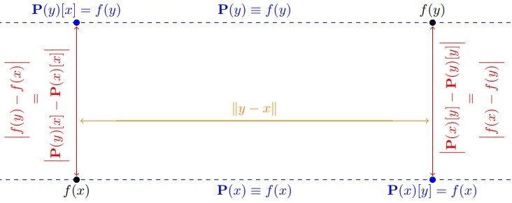
In the diagram above we fix $x,y \in \mathbb{R}$ and consider a $\gamma$-Hőlder continuous $f : \{ x , y \} \to \mathbb{R}$. As illustrated by the $\color{Blue}{blue}$ dotted lines, we define a function $\textbf{P} : \{ x , y \} \to \mathrm{Poly}_0\big( \mathbb{R}^d;\mathbb{R} \big)$ by $\textbf{P}(x) \equiv f(x)$ and $\textbf{P}(y) \equiv f(y)$. The diagram then illustrates the equivalency of the estimates in \eqref{eq:gamma_holder_cont_def} and \eqref{eq:refined_gamma_holder_cont}. The $\color{red}{red}$ arrows show the value $\big\vert f(y) - f(x) \big\vert = \big\vert \textbf{P}(x)[y] - \textbf{P}(y)[y] \big\vert = \big\vert \textbf{P}(y)[x] - \textbf{P}(x)[x] \big\vert$ that is required to be controlled from above by the quantity $\Vert y - x \Vert$, illustrated by the $\color{orange}{orange}$ arrow, raised to the power of $\gamma \in (0,1]$.
In [Stein, 1970], Stein generalises the notion of $\gamma$-Hőlder continuity determined, for $\gamma \in (0,1]$, by the estimates \eqref{eq:refined_gamma_holder_cont} to the case of a general $\gamma > 0$ (in particular, allowing for the possibility that $\gamma > 1$). Loosely, Stein's approach is to mimic Whitney's approach with the little-o estimates on the difference between the derivatives of various polynomials imposed in \eqref{eq:whitney_CkA_cond} replaced with big-O variants that are more reflective of the $\mathcal{O} \big( \Vert y - x \Vert^{\gamma} \big)$ estimate required in \eqref{eq:refined_gamma_holder_cont}.
To make this more precise, fix a closed subset $A \subset \mathbb{R}^d$ and fix a choice of $\gamma > 0$. Let $k \in \mathbb{Z}_{\geqslant 0}$ for which $\gamma \in (k,k+1]$. Then one interpretation of Stein's definition of the class $\mathrm{Lip}(\gamma,A,\mathbb{R})$ is as follows. The space $\mathrm{Lip}(\gamma,A,\mathbb{R})$ consists of all functions $\textbf{P} : A \to \mathrm{Poly}_k(\mathbb{R}^d;\mathbb{R})$ for which there exists a constant $C \geqslant 0$ such that for every $l \in \{0 , \ldots , k\}$ and every $x,y \in A$ we have that \begin{equation} \tag{12}\label{eq:Stein_Lip_gamma_conds_v1} \Bigg\Vert \Big( D^l_{\omega}\textbf{P}(x)[\omega] \Big)\Big\vert_{\omega = x} \Bigg\Vert_{\rm{op}} \leqslant C \qquad \text{and} \qquad \Bigg\Vert\Big( D^l_{\omega} \Big( \textbf{P}(y)[\omega] - \textbf{P}(x)[\omega] \Big)\Big)\Big\vert_{\omega = y} \Bigg\Vert_{\rm{op}} \leqslant C \Vert y - x \Vert^{\gamma -l}. \end{equation} An equivalent definition involving a more traditional notion of a function $A \to \mathbb{R}$ can be arrived at as follows. Observe, for each $x \in A$, that $\textbf{P}(x)$ is a degree $k$ polynomial $\mathbb{R}^d \to \mathbb{R}$. Consequently, Taylor's Theorem tells us, for any $y \in A$, that \begin{equation} \tag{13}\label{eq:Tay_expand_deg_k_poly_A} \textbf{P}(x)[y] = \sum_{s=0}^k \frac{1}{s!} \Big( D^s_{\omega}\textbf{P}(x)[\omega] \Big)\Big\vert_{\omega = x} \Big[ \big( y - x \big)^{\otimes s} \Big]. \end{equation} Define $f^{(0)} : A \to \mathbb{R}$ by setting $f^{(0)}(x) := \textbf{P}(x)[x]$ for each $x \in A$. Further, if $k \geqslant 1$, for each $s \in \{1, \ldots , k\}$ define $f^{(s)} : A \to \mathcal{L} \Big( \big( \mathbb{R}^d \big)^{\otimes s}; \mathbb{R} \Big)$ by setting $f^{(s)}(x) := \Big( D^s_{\omega}\textbf{P}(x)[\omega] \Big)\Big\vert_{\omega = x}$ for each $x \in A$. It follows that \eqref{eq:Tay_expand_deg_k_poly_A} may be expressed as \begin{equation} \tag{14}\label{eq:Tay_expand_deg_k_poly_B} \textbf{P}(x)[y] = \sum_{s=0}^k \frac{1}{s!} f^{(s)}(x) \Big[ \big( y - x \big)^{\otimes s} \Big]. \end{equation} Together, \eqref{eq:Tay_expand_deg_k_poly_B} and direct computation yield, for each $l \in \{0 , \ldots , k\}$, any $x,y \in A$, and any $v \in \big( \mathbb{R}^d \big)^{\otimes l}$, that \begin{equation} \tag{15}\label{eq:poly_deriv_diff_remainder_form_A} \Big( D^l_{\omega} \Big( \textbf{P}(y)[\omega] - \textbf{P}(x)[\omega] \Big) \Big)\Big\vert_{\omega = y} [v] = f^{(l)}(y)[ v ] - \sum_{s=0}^{k-l} \frac{1}{s!} f^{(l+s)}(x) \Big[ v \otimes (y - x)^{\otimes s} \Big]. \end{equation} Motivated by \eqref{eq:poly_deriv_diff_remainder_form_A}, for each $s \in \{0, \ldots , k\}$ we introduce the remainder term $R^f_s : A \times A \to \mathcal{L} \Big( \big( \mathbb{R}^d \big)^{\otimes s} ; \mathbb{R} \Big)$ as follows. For $x,y \in A$ we define \begin{equation}\tag{16}\label{eq:0_remain_term_def} R^f_0(x,y) := f^{(0)}(y) - \sum_{j=0}^k \frac{1}{j!} f^{(j)}(x) \Big[ (y-x)^{\otimes j} \Big].\end{equation} For $s \in \{1, \ldots ,k\}$, any $x,y \in A$, and any $v \in \big( \mathbb{R}^d \big)^{\otimes s}$ we define \begin{equation} \tag{17}\label{eq:s_remain_term_def} R^f_s(x,y)[v] := f^{(s)}(y)[v] - \sum_{j=0}^{k-s} \frac{1}{j!} f^{(s+j)}(x) \Big[ v \otimes (y-x)^{\otimes j} \Big]. \end{equation} The combination of \eqref{eq:poly_deriv_diff_remainder_form_A}, \eqref{eq:0_remain_term_def}, and \eqref{eq:s_remain_term_def} yields that the estimates in \eqref{eq:Stein_Lip_gamma_conds_v1} are equivalent to having, for every $l \in \{0, \ldots , k\}$ and every $x,y \in A$, that \begin{equation} \tag{18}\label{eq:Stein_Lip_gamma_conds_v2} \Big\Vert f^{(l)}(x) \Big\Vert_{\rm{op}} \leqslant C \qquad \text{and} \qquad \Big\Vert R^f_l(x,y) \Big\Vert_{\rm{op}}\leqslant C \Vert y - x \Vert^{\gamma - l}. \end{equation} Consequently, one can equivalently view $\mathrm{Lip}(\gamma,A,\mathbb{R})$ as $f = \big( f^{(0)}, \ldots , f^{(k)} \big)$ where, for each $l \in \{0, \ldots ,k\}$, $f^{(l)} : A \to \mathcal{L} \Big( \big( \mathbb{R}^d \big)^{\otimes l} ; \mathbb{R}\Big)$ is a mapping into the space of symmetric $l$-linear forms from $\mathbb{R}^d$ to $\mathbb{R}$, and such that the mappings $f^{(0)} , \ldots , f^{(k)}$ and the remainder terms $R^f_0 , \ldots , R^f_k$, as defined in \eqref{eq:0_remain_term_def} and \eqref{eq:s_remain_term_def} respectively, satisfy the estimates detailed in \eqref{eq:Stein_Lip_gamma_conds_v2}. The smallest constant $C \geqslant 0$ for which the estimates \eqref{eq:Stein_Lip_gamma_conds_v2} (equivalently \eqref{eq:Stein_Lip_gamma_conds_v1}) are valid is defined to be the $\mathrm{Lip}(\gamma,A,\mathbb{R})$ norm of $f$ (equivalently of $\textbf{P}$) and denoted by $\Vert f \Vert_{\mathrm{Lip}(\gamma,A,\mathbb{R})}$ or $\Vert \textbf{P} \Vert_{\mathrm{Lip} (\gamma,A,\mathbb{R})}$ depending on the viewpoint adopted. We will often refer to $\mathrm{Lip}(\gamma,A,\mathbb{R})$ as the set of real-valued $\mathrm{Lip} (\gamma)$ functions defined on $A$. When equipped with the norm $\Vert \cdot \Vert_{\mathrm{Lip}(\gamma,A,\mathbb{R})}$, the space $\mathrm{Lip} (\gamma,A,\mathbb{R})$ becomes a Banach space.
This latter formulation is more reminiscent of Whitney's original definition of a function $A \to \mathbb{R}$ being of class $C^m$ for some $m \in \mathbb{Z}_{\geqslant 1}$. Indeed if $f = \big( f^{(0)}, \ldots , f^{(k)} \big) \in \mathrm{Lip}(\gamma,A,\mathbb{R})$ then, for each $l \in \{1, \ldots , k\}$, the quantity $f^{(l)}(x)$ gives a proposal for the $l^{\text{th}}$ derivative of $f^{(0)}$ at the point $x \in A$. This motivates the commonly adopted notation of dropping the superscript $(0)$ from $f^{(0)}$ and referring to $f: A \to \mathbb{R}$ as a $\mathrm{Lip}(\gamma)$ function without explicit reference to the corresponding $f^{(1)}, \ldots , f^{(k)}$. To avoid potential confusion we will not use this notation unless $\gamma \in (0,1]$, in which case this viewpoint of a $\mathrm{Lip}(\gamma,A,\mathbb{R})$ function involves only a single function $A \to \mathbb{R}$ anyway. In the case that $\gamma > 1$, if we refer to $f \in \mathrm{Lip}(\gamma,A,\mathbb{R})$ then the underlying function $A \to \mathbb{R}$ will always be denoted as $f^{(0)}$.
To illustrate Stein's notion of $\mathrm{Lip}(\gamma,A,\mathbb{R})$ we present an explicit example in the setting that $d:=1$, $A := \{0,1/2\} \subset \mathbb{R}$, and $\gamma := 4$. Consider the mapping $\textbf{P} : A \to \mathrm{Poly}_3(\mathbb{R};\mathbb{R})$ defined, for $x \in A$ and $t \in \mathbb{R}$, by \begin{equation} \tag{19}\label{eq:lip_4_example_poly_def} \textbf{P}(x)[t] := \Bigg\{ \begin{array}{ccc} 2 t^3 - 2 t^2 + 3t + 2 & \text{if} & x=0 \\ -\big( t - \frac{1}{2} \big)^3 + 4\big(t-\frac{1}{2}\big)^2 - 2\big( t - \frac{1}{2} \big) + 4 & \text{if} & x=\frac{1}{2}. \end{array} \end{equation} This corresponds to considering the polynomial $P_1(t) := 2 t^3 - 2 t^2 + 3t + 2$ based at $x=0$, and the polynomial $P_2(t) := -\big( t - \frac{1}{2} \big)^3 + 4\big(t-\frac{1}{2}\big)^2 - 2\big( t - \frac{1}{2} \big) + 4$ based at $x=1/2$. Computation of the derivatives of $P_1$ and $P_2$ establishes that this is equivalent to considering $f^{(0)} : A \to \mathbb{R}$ defined, for $x \in A$, by \begin{equation} \tag{20}\label{eq:lip_4_example_f0} f^{(0)}(x) := \Bigg\{ \begin{array}{ccc} 2 & \text{if} & x=0 \\ 4 & \text{if} & x=\frac{1}{2}, \end{array} \end{equation} considering $f^{(1)} : A \to \mathcal{L}(\mathbb{R};\mathbb{R})$ defined, for $x \in A$ and $v \in \mathbb{R}$, by \begin{equation} \tag{21}\label{eq:lip_4_example_f1} f^{(1)}(x)[v] := \Bigg\{ \begin{array}{ccc} 3v & \text{if} & x=0 \\ -2v & \text{if} & x=\frac{1}{2}, \end{array} \end{equation} considering $f^{(2)} : A \to \mathcal{L}\big(\mathbb{R}^{\otimes 2};\mathbb{R}\big)$ defined, for $x \in A$ and $v_1 , v_2 \in \mathbb{R}$, by \begin{equation} \tag{22}\label{eq:lip_4_example_f2} f^{(2)}(x)\big[v_1 \otimes v_2 \big] := \Bigg\{ \begin{array}{ccc} -4v_1v_2 & \text{if} & x=0 \\ 8v_1v_2 & \text{if} & x=\frac{1}{2}, \end{array} \end{equation} and considering $f^{(3)} : A \to \mathcal{L} \big(\mathbb{R}^{\otimes 3};\mathbb{R}\big)$ defined, for $x \in A$ and $v_1 , v_2 , v_3 \in \mathbb{R}$, by \begin{equation} \tag{23}\label{eq:lip_4_example_f3} f^{(3)}(x)\big[v_1 \otimes v_2 \otimes v_3 \big] := \Bigg\{ \begin{array}{ccc} 12v_1v_2v_3 & \text{if} & x=0 \\ -6v_1v_2v_3 & \text{if} & x=\frac{1}{2}. \end{array} \end{equation} It follows from \eqref{eq:lip_4_example_f0}, \eqref{eq:lip_4_example_f1}, \eqref{eq:lip_4_example_f2}, and \eqref{eq:lip_4_example_f3} that \begin{equation} \tag{24}\label{eq:lip_4_example_ptwse_norm_bds} \max_{j \in \{0,1,2,3\}} \max_{x \in A} \Big\Vert f^{(j)}(x) \Big\Vert_{\rm{op}} = 12. \end{equation} The remainder term considerations for computing the $\mathrm{Lip}(4,\{0,1/2\},\mathbb{R})$ norm of $f := \big( f^{(0)} , f^{(1)} , f^{(2)} , f^{(3)} \big)$, or, equivalently, of the mapping $\textbf{P} : \{0,1/2\} \to \mathrm{Poly}_3(\mathbb{R};\mathbb{R})$, are illustrated in the diagram at the end of this section. This task requires computing the remainder terms $R_0^f, R^f_1, R^f_2$, and $R^f_3$ as defined in \eqref{eq:0_remain_term_def} and \eqref{eq:s_remain_term_def} respectively. Recalling \eqref{eq:poly_deriv_diff_remainder_form_A} we can compute that \begin{equation} \tag{25}\label{eq:lip_4_example_remain_bds} \begin{array}{cc} \Big\Vert R^f_0 \big( 0 , \frac{1}{2} \big) \Big\Vert_{\rm{op}} = \frac{33}{8} = 66\Big( \frac{1}{2} \Big)^4 & \Big\Vert R^f_0 \big( \frac{1}{2} , 0 \big) \Big\Vert_{\rm{op}} = \frac{3}{4} = 12\Big( \frac{1}{2} \Big)^4 \\ \Big\Vert R^f_1 \big( 0 , \frac{1}{2} \big) \Big\Vert_{\rm{op}} = \frac{39}{4} = 78\Big( \frac{1}{2} \Big)^3 & \Big\Vert R^f_1 \big( \frac{1}{2} , 0 \big) \Big\Vert_{\rm{op}} = \frac{9}{2} = 36 \Big( \frac{1}{2} \Big)^3 \\ \Big\Vert R^f_2 \big( 0 , \frac{1}{2} \big) \Big\Vert_{\rm{op}} = 15 = 60\Big( \frac{1}{2} \Big)^2 & \Big\Vert R^f_2 \big( \frac{1}{2} , 0 \big) \Big\Vert_{\rm{op}} = 6 = 24\Big( \frac{1}{2} \Big)^2 \\ \Big\Vert R^f_3 \big( 0 , \frac{1}{2} \big) \Big\Vert_{\rm{op}} = 18 = 36\Big( \frac{1}{2} \Big) & \Big\Vert R^f_3 \big( \frac{1}{2} , 0 \big) \Big\Vert_{\rm{op}} = 18 = 36\Big( \frac{1}{2} \Big). \end{array} \end{equation} Together, \eqref{eq:lip_4_example_ptwse_norm_bds} and \eqref{eq:lip_4_example_remain_bds} yield that \begin{equation} \tag{26}\label{eq:lip_4_example_lip_4_norm} \big\Vert f \big\Vert_{\mathrm{Lip}(4,\{0,1/2\},\mathbb{R})} = 78. \end{equation}
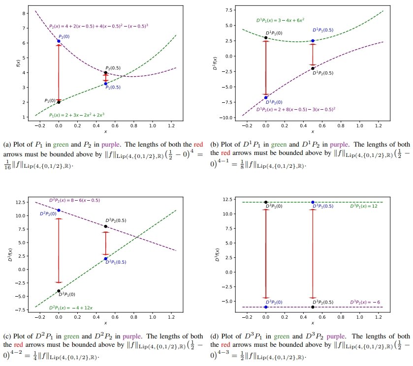
Plots illustrating the comparison of the derivatives of $P_1$ and $P_2$ and how the differences relate to the norm $\Vert f \Vert_{\mathrm{Lip}(4,\{0,1/2\},\mathbb{R})}$. In each Sub-Figure the size of the $\color{red}{red}$ arrows is required to be controlled by the norm $\Vert f \Vert_{\mathrm{Lip}(4,\{0,1/2\},\mathbb{R})}$ multiplied by the distance between $0$ and $\frac{1}{2}$ raised to an appropriate power; i.e. controlled by $2^{-j}\Vert f \Vert_{\mathrm{Lip}(4,\{0,1/2\},\mathbb{R})}$ for $j=1,2,3,4$ respectively.
We next return to the general setting of considering a closed subset $A \subset \mathbb{R}^d$ for some integer $d \in \mathbb{Z}_{\geqslant 1}$, and remark on how Stein's class $\mathrm{Lip}(\gamma,A,\mathbb{R})$ relates to more familiar notions of regularity.
First, we suppose that $\gamma \in (0,1]$. In this case an element in $\mathrm{Lip}(\gamma,A,\mathbb{R})$ may be viewed as either a mapping $\textbf{P} : A \to \mathrm{Poly}_0(\mathbb{R}^d;\mathbb{R})$, or equivalently as a single function $f^{(0)} : A \to \mathbb{R}$. As stated previously, the relationship between these two equivalent viewpoints is that for every $x \in A$ we have $f^{(0)}(x) = \textbf{P}(x)[x]$. In this case we have that the remainder term $R_0^f : A \times A \to \mathbb{R}$ is given, for $x,y \in A$, by $R_0^f(x,y) = f^{(0)}(y) - f^{(0)}(x)$. The estimates required in \eqref{eq:Stein_Lip_gamma_conds_v2} yield that $f^{(0)}$ is a bounded $\gamma$-Hőlder continuous function $A \to \mathbb{R}$. Consequently, when $\gamma \in (0,1]$ we have \begin{equation} \tag{27}\label{eq:gamma_in_(0,1]_equiv} \mathrm{Lip}(\gamma,A,\mathbb{R}) = C^{0,\gamma}(A). \end{equation} Secondly, suppose that $O \subset \mathbb{R}^d$ is an open subset. A verbatim repetition of Stein's definition with the closed subset $A$ replaced with the open subset $O$ enables us to consider the class $\mathrm{Lip}(\gamma,O,\mathbb{R})$ of real-valued $\mathrm{Lip}(\gamma)$ functions defined on $O$. Let $f = \Big( f^{(0)} , \ldots , f^{(k)} \Big) \in \mathrm{Lip}(\gamma,O,\mathbb{R})$. The definitions of the remainder terms $R_0^f , \ldots , R^f_k$, given in \eqref{eq:0_remain_term_def} and \eqref{eq:s_remain_term_def} respectively, and the bounds in \eqref{eq:Stein_Lip_gamma_conds_v2} establish that $f^{(0)} : O \to \mathbb{R}$ is $k$-times Fréchet differentiable in the classical sense, and that for each $l \in \{0 , \ldots , k\}$ we have that $D^l f^{(0)} \equiv f^{(l)}$ throughout $O$. In particular, \eqref{eq:Stein_Lip_gamma_conds_v2} yields that $f^{(0)} , \ldots , D^k f^{(0)}$ are all bounded, and that the $k^{\text{th}}$ derivative $D^k f^{(0)}$ is $(\gamma-k)$-Hőlder continuous since, for $x,y \in O$, we have $D^k f^{(0)}(y) - D^k f^{(0)}(x) = f^{(k)}(y) - f^{(k)}(x) = R^f_k(x,y)$. Consequently, if $O \subset \mathbb{R}^d$ is open and $C^{k,\gamma-k}(O)$ denotes the set of $k$-times Fréchet differentiable functions $O \to \mathbb{R}$ with $(\gamma - k)$-Hőlder continuous $k^{\text{th}}$ derivative, we have \begin{equation} \tag{28}\label{eq:O_open_equiv} \mathrm{Lip}(\gamma,O,\mathbb{R}) = C^{k,\gamma - k}_b(O) := \Big\{ \psi \in C^{k,\gamma-k}(O) ~\big\vert~ \psi , \ldots , D^k \psi \text{ all bounded} \Big\}. \end{equation} This observation has impact on the class $\mathrm{Lip}(\gamma,A,\mathbb{R})$ for a closed subset $A \subset \mathbb{R}^d$. Indeed, the interior of $A$, denoted $\rm{Interior}(A)$, is a (possibly empty) open subset of $\mathbb{R}^d$. Thus, via \eqref{eq:O_open_equiv} with $O := \rm{Interior}(A)$, if $f = \Big( f^{(0)} , \ldots , f^{(k)} \Big) \in \mathrm{Lip}(\gamma,A,\mathbb{R})$ we always have that $f^{(0)} \in C^{k,\gamma-k}_b \big( \rm{Interior}(A) \big)$ with, for each $l \in \{0, \ldots , k\}$, $D^l f^{(0)} \equiv f^{(l)}$ throughout $\rm{Interior}(A)$. However, at points not in the interior $\rm{Interior}(A)$, there is no requirement that the functions $f^{(1)} , \ldots , f^{(k)}$ are uniquely determined by the function $f^{(0)}$.
Finally, once again consider a closed subset $A \subset \mathbb{R}^d$ and an element $f = \Big( f^{(0)} , \ldots , f^{(k)} \Big) \in \mathrm{Lip}(\gamma,A,\mathbb{R})$. As observed previously, for every $x,y \in A$ we have that $f^{(k)}(y) - f^{(k)}(x) = R_k^f(x,y)$. Consequently, the bounds \eqref{eq:Stein_Lip_gamma_conds_v2} for $l := k$ establish that the function $f^{(k)} : A \to \mathcal{L} \Big( \big( \mathbb{R}^d \big)^{\otimes k};\mathbb{R} \Big)$ is always bounded and $(\gamma-k)$-Hőlder continuous.
In addition to its sensible interaction with more familiar notions of higher order regularity, Stein's notion of $\mathrm{Lip}(\gamma)$ regularity satisfies the following properties that make it an attractive function class from a Machine Learning perspective.
- Higher Order Regularity on Arbitrary Closed Subsets: $\mathrm{Lip}(\gamma)$ regularity gives a notion of smoothness that is well-defined on any closed subset including, in particular, finite subsets. In Machine Learning it is often the case that we only know a systems response to a finite number of observed inputs; and that the goal is to use these known responses to learn how to predict the systems response to new unseen inputs. $\mathrm{Lip}(\gamma)$ functions provide a way to define smooth functions on such finite data sets without making any artificial assumption at points outside the given subset. The function is only constrained at the inputs for which the systems response is known; no values are prescribed at inputs for which the systems response is not known.
- Universal Nonlinearity: It is known that the product of two real-valued $\mathrm{Lip}(\gamma)$ functions is itself a real-valued $\mathrm{Lip} (\gamma)$ function; see, for example, Proposition 1.38 in [Boutaib, 2020] for a more general version of this result. Hence real-valued $\mathrm{Lip}(\gamma)$ functions span an algebra. Consequently, via the Stone-Weierstrass Theorem [Stone, 1948], on compact subsets any real-valued continuous function can be well-approximated by a linear combination of real-valued $\mathrm{Lip}(\gamma)$ functions. Thus the class of real-valued $\mathrm{Lip}(\gamma)$ functions satisfies the universality property that, on compact subsets, it is rich enough to capture any continuous system.
Inference: Stein proves that $\mathrm{Lip}(\gamma)$ functions satisfy an extension theorem (cf. Theorem 4 in Chapter VI of [Stein, 1970]) analogous to the extension theorem established by Whitney in [Whitney, 1934a] (cf. Theorem I in [Whitney, 1934a]). We adopt the terminology Stein-Whitney Extension Theorem to reflect the fundamental reliance of Stein's proof in [Stein, 1970] on the original machinery and tools developed by Whitney in [Whitney, 1934a].
Stein-Whitney Extension Theorem (Chapter VI, Theorem 4 in [Stein, 1970]) Let $d \in \mathbb{Z}_{\geqslant 1}$, $A \subset \mathbb{R}^d$ closed, and $\gamma > 0$ with $k \in \mathbb{Z}_{\geqslant 0}$ such that $\gamma \in (k,k+1]$. Then there exists a constant $C = C(\gamma,d) \geqslant 1$ such that given any $f \in \mathrm{Lip}(\gamma,A,\mathbb{R})$ there exists $F \in \mathrm{Lip}(\gamma,\mathbb{R}^d,\mathbb{R}) = C^{k,\gamma-k}_b \big( \mathbb{R}^d \big)$ with $F \big\vert_A \equiv f$ and $\Vert F \Vert_{\mathrm{Lip}(\gamma,\mathbb{R}^d,\mathbb{R})} \leqslant C \Vert f \Vert_{\mathrm{Lip}(\gamma,A,\mathbb{R})}$.
A particular consequence of the Stein-Whitney Extension Theorem is that given any $f \in \mathrm{Lip}(\gamma,A,\mathbb{R})$ and any point $p \in \mathbb{R}^d \setminus A$, one may extend $f$ so that it remains within the class of $\mathrm{Lip}(\gamma)$ regularity, and is now additionally defined at $p$. This means that any $\mathrm{Lip}(\gamma)$ regular model can be extended within the same regularity class for the purpose of inference on any new input. This regularity class preservation is essential to the introduction of Log-NCDEs in [Walker et al., 2024].
In [Lyons & McLeod, 2024a] we consider the local behaviour of extensions of a given $\mathrm{Lip}(\gamma)$ function. More precisely, we suppose that $A,B \subset \mathbb{R}^d$ are closed subsets with $B \subset A$. Given $f \in \mathrm{Lip}(\gamma,B,\mathbb{R})$, a consequence of the Stein-Whitney Extension Theorem is that $f$ can be extended to a function $F \in \mathrm{Lip}(\gamma,A,\mathbb{R})$. In general, there is no uniqueness associated to the extension. For example, take $d := 1$ and consider $B := [-1/2,1/2]$ and $A := [-1,1]$. Then the mapping $B \to \mathbb{R}$ given by $x \mapsto \vert x \vert$ determines a function in $\mathrm{Lip}(1,B,\mathbb{R})$, and there are numerous distinct ways it can be extended to a function in $\mathrm{Lip}(1,A,\mathbb{R})$. However, it seems intuitively clear that any two extensions must be, in some sense, close for points $x \in [-1,1]$ that are not, in some sense, too far away from $[-1/2,-1/2]$.
The Lipschitz Sandwich Theorems established in [Lyons & McLeod, 2024a] provide precise realisations of this intuition. They can loosely be summarised by the following informal principle. Given closed subsets $A,B \subset \mathbb{R}^d$ with $B \subset A$, the following implication is true: \begin{equation} \tag{29}\label{eq:HOLST_summary} \begin{array}{ccc} \psi , \varphi \in \mathrm{Lip}(\gamma,A,\mathbb{R}) & & \\ \psi \equiv \varphi \text{ throughout } B & \implies & \begin{array}{c} \psi \text{ and } \varphi \text{ close in } \mathrm{Lip}(\eta) \text{ norm sense at} \\ \text{points within a definite distance of } B. \end{array} \\ \eta \in (0,\gamma) & & \end{array} \end{equation} The restriction that $\eta < \gamma$ is essential; the implication \eqref{eq:HOLST_summary} is, in general, not true for $\eta := \gamma$. To illustrate, consider $d=1$ and $B := \{0\} \subset \mathbb{R}$ and $A := [0,1] \subset \mathbb{R}$. Define $\psi , \varphi : [0,1] \to \mathbb{R}$ by, for $t \in [0,1]$, $\psi(t) := 0$ and $\varphi(t) := t$. Then $\psi, \varphi \in \mathrm{Lip}(1,A,\mathbb{R})$, $\psi \equiv \varphi$ throughout $B$, but for any $\delta \in (0,1/2)$, say, we have that $\Vert \psi - \varphi \Vert_{\mathrm{Lip}(1,[0,\delta],\mathbb{R})} = 1$.
The requirement that $\psi$ and $\varphi$ coincide throughout $B$ can be weakened to requiring that the functions $\psi^{(0)}$ and $\varphi^{(0)}$, and their respective proposed derivatives $\psi^{(1)}, \ldots , \psi^{(k)}$ and $\varphi^{(1)}, \ldots , \varphi^{(k)}$ in the case that $k \geqslant 1$, are close in a pointwise sense throughout $B$; see the Lipschitz Sandwich Theorem 3.1 in [Lyons & McLeod, 2024a].
We illustrate the intuition behind the Sandwich Theorems obtained in [Lyons & McLeod, 2024a] in the diagram at the end of this section. For this purpose, we take $d := 1$, $A := [0,0.7] \subset \mathbb{R}$, $B := \{0.3\} \subset \mathbb{R}$, and $\gamma := 4$. Then $P_1 : [0,0.7] \to \mathbb{R}$ defined, for $x \in \mathbb{R}$, by $P_1(x) := 10(x-0.3)^3 - 8(x-0.3)^2 + 5$ determines \begin{equation} \tag{30}\label{eq:bold_P1} \textbf{P}_1 := \Big( P_1 , D^1P_1 , D^2P_1 , D^3 P_1 \Big) \in \mathrm{Lip}(4,[0,0.7],\mathbb{R}). \end{equation} Our aim is to consider example $\mathrm{Lip}(4,[0,0.7],\mathbb{R})$ functions that coincide with $\textbf{P}_1$ on $B$, i.e. at the point $x=0.3$. Recalling \eqref{eq:O_open_equiv} and \eqref{eq:bold_P1}, any function $f \in C^{3,1}([0,0.7])$ with $f(0.3) = P_1(0.3)$, $D^1 f(0.3) = D^1 P_1(0.3)$, $D^2 f(0.3) = D^2P_1(0.3)$, and $D^3f(0.3) = D^3 P_1(0.3)$ determines \begin{equation} \tag{31}\label{eq:bold_f} \textbf{f} := \Big( f , D^1 f , D^2 f , D^3 f \Big) \in \mathrm{Lip}(4,[0,0.7],\mathbb{R}) \end{equation} satisfying that $\textbf{f} \equiv \textbf{P}_1$ throughout $B$. For simplicity, we restrict to considering such functions $f:[0,0.7] \to \mathbb{R}$ that are polynomials of the form $x \mapsto P_1(x) + \mathcal{O} \big( (x-0.3)^4 \big)$. In particular, we consider $P_2,P_3,P_4 : [0,0.7] \to \mathbb{R}$ defined, for $x \in [0,0.7]$, by \begin{equation} \tag{32}\label{eq:P2P3P4} \begin{array}{c} P_2(x) := P_1(x) + 15(x-0.3)^4 -50(x-0.3)^6 \\ P_3(x) := P_1(x) -10(x-0.3)^4 + 40(x-0.3)^9 \\ P_4(x) := P_1(x) + 40(x-0.3)^4 \end{array} \end{equation} so that the corresponding \begin{equation} \tag{33}\label{eq:bP2bP3bP4} \begin{array}{c} \textbf{P}_2 = \Big( P_2 , D^1 P_2 , D^2 P_2 , D^3 P_2 \Big) \in \mathrm{Lip}(4, [0,0.7] , \mathbb{R}) \\ \textbf{P}_3 = \Big( P_3 , D^1 P_3 , D^2 P_3 , D^3 P_3 \Big) \in \mathrm{Lip}(4, [0,0.7] , \mathbb{R}) \\ \textbf{P}_4 = \Big( P_4 , D^1 P_4 , D^2 P_4 , D^3 P_4 \Big) \in \mathrm{Lip}(4, [0,0.7] , \mathbb{R}) \end{array} \end{equation} satisfy $\textbf{P}_1 \equiv \textbf{P}_2 \equiv \textbf{P}_3 \equiv \textbf{P}_4$ throughout $B = \{0.3\}$.
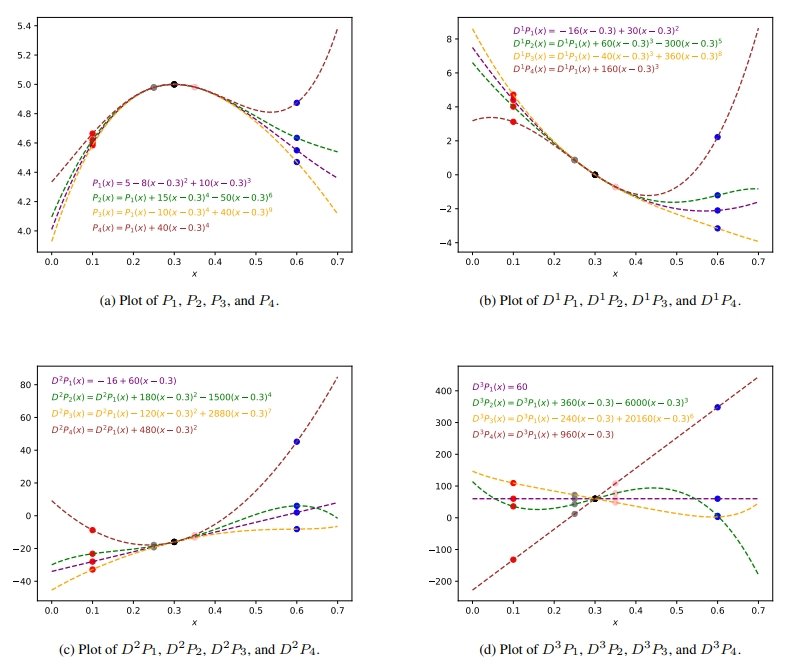
The Sub-Figures (a), (b), (c), and (d) display plots the derivatives (up to third-order) of the polynomials $P_1$, $P_2$, $P_3$, and $P_4$ for points $x \in [0,0.7]$. Each plot illustrates the intuition behind the Lipschitz Sandwich Theorems established in [Lyons & McLeod, 2024a]; whilst the functions can differ significantly at points far away from $x=0.3$, illustrated by the $\color{red}{red}$ and $\color{blue}{blue}$ dots in each plot, they are all forced to become much closer to one and other at points close to $x=0.3$, illustrated by the $\color{gray}{grey}$ and $\color{pink}{pink}$ in each plot.
However, it is not just the pointwise values that influence the Lipschitz norm; indeed, the remainder terms (cf. \eqref{eq:0_remain_term_def} and \eqref{eq:s_remain_term_def}) mean that the gradients of each graph affect the Lipschitz norm. That the gradients for the derivatives up to second-order, shown in Sub-Figures (a), (b), and (c) respectively, become almost indistinguishable on small intervals about $x=0.3$ illustrates that for any given $\eta \in (0,3]$, by choosing a sufficiently small $\delta > 0$, we can, for any $i,j \in \{1, 2, 3, 4\}$, make the $\mathrm{Lip}(\eta,[0.3-\delta,0.3+\delta],\mathbb{R})$ norm of the difference $\textbf{P}_i - \textbf{P}_j$ arbitrarily small.
Sub-Figure (d) illustrates that whilst this remains true for $\eta \in (3,4)$, it is in fact not possible for $\eta := 4$. The issue is that the gradients of each plot no longer coincide at $x=0.3$. Observe that the $\mathrm{Lip}(4,[0.3-\delta,0.3+\delta],\mathbb{R})$ norm of $\textbf{P}_1 - \textbf{P}_4$ is at least as large as the smallest constant $C \geqslant 0$ for which \begin{equation} \tag{34}\label{eq:Lip4_norm_LB} \Big\Vert D^3(P_1 - P_4)(0.3 + \delta) - D^3(P_1 - P_4)(0.3) \Big\Vert_{\rm{op}} \leqslant C \delta \end{equation} But direct computation shows that $D^3(P_1 - P_4)(0.3 + \delta) - D^3(P_1 - P_4)(0.3) = 960 \delta$, hence the smallest constant $C$ so that \eqref{eq:Lip4_norm_LB} is valid is $C := 960$. Consequently we must have that \begin{equation} \tag{35}\label{eq:Lip4_norm_not_small} \big\Vert \textbf{P}_1 - \textbf{P}_4 \big\Vert_{ \mathrm{Lip}(4, [0.3-\delta,0.3+\delta],\mathbb{R})} \geqslant 960 \end{equation} irrespective of the size of $\delta > 0$. Observe that this issue can be overcome provided we restrict to $\eta \in (3,4)$; in this case the bound required in \eqref{eq:Lip4_norm_LB} is $C \delta^{\eta - 3}$ and so we have an extra $\delta^{1-(\eta-3)}$ factor in \eqref{eq:Lip4_norm_not_small}. Thus the equivalent lower bound to the lower bound \eqref{eq:Lip4_norm_not_small} for the $\mathrm{Lip}(\eta,[0.3-\delta,0.3+\delta],\mathbb{R})$ norm of $\textbf{P}_1 - \textbf{P}_4$ is $960 \delta^{1-(\eta-3)}$, and evidently this can be made arbitrarily small by choosing $\delta$ suitably small.
Observe that the size of interval about $x=0.3$ on which the derivatives of $P_1$, $P_2$, $P_3$, and $P_4$ remain close decreases as the order of derivative considered increases. This reflects the, loosely stated, phenomena that the size of the neighbourhood of $x=0.3$ on which the $\mathrm{Lip}(\eta)$ norm is small is decreasing as a function of $\eta \in (0,\gamma)$. Higher order Lipschitz control requires restricting to smaller neighbourhoods of the subset $B$. The size of the neighbourhood on which such control can be established also depends on $\gamma - \eta$; larger values of this difference result in larger neighbourhoods on which the smallness of the $\mathrm{Lip}(\eta)$ norm can be guaranteed. Further precise details can be found in [Lyons & McLeod, 2024a].
In this particular example, the consequences of the Lipschitz Sandwich Theorems from [Lyons & McLeod, 2024a] are easily established. We have that functions in $\mathrm{Lip}(4,[0,0.7],\mathbb{R})$ are functions in $C^{3,1}([0,0.7])$, and so the functions involved have classical derivatives of order $\leqslant 3$. This enables one to deduce the required estimates via the Fundamental Theorem of Calculus. The main content of [Lyons & McLeod, 2024a] is establishing that this expected phenomenon remains valid in situations in which the classical derivatives do not exist. This, in particular, includes the more usual Machine Learning setting in which both the subsets $A$ and $B$ are finite; that is, the setting in which we consider extensions of a $\mathrm{Lip}(\gamma)$ function from one finite subset of inputs to a second, larger finite subset of inputs.
The Lipschitz Sandwich Theorems obtained in [Lyons & McLeod, 2024a] underpin further properties of $\mathrm{Lip}(\gamma)$ functions that are attractive from a Machine Learning perspective, including the following.
- Quantitative Inference: Under the assumption that the system of interest satisfies some weak global $\mathrm{Lip}(\gamma)$ regularity, the Lipschitz Sandwich Theorems yield quantitative inference estimates. In particular, one can estimate the error made by a $\mathrm{Lip}(\gamma)$ model when used for inference on a new unseen input in terms of the distance between the new input and the collection of previously observed inputs for which the systems response is known.
- Cost-Effective Approximation: The behaviour of a $\mathrm{Lip}(\gamma)$ function on a non-empty compact set is determined by its values at a finite number $N \in \mathbb{Z}_{\geqslant 1}$ of points. The integer $N$ depends on, amongst other things, the covering number, in the sense of Kolmogorov [Kolmogorov, 1956], of the compact set. As the regularity parameter $\gamma > 0$ increases the integer $N$ decreases. See Section 4 in [Lyons & McLeod, 2024a].
Sparse-Approximation of Linear Combinations: Linear combinations of functions are ubiquitous in Machine Learning; as an example, each layer of a neural network may be viewed as a linear combination of functions. Sparse approximations of such linear combinations offer an approach to inference acceleration via reduction of a models computational complexity. Loosely, a sparse approximation in this context means the following. Given $\varphi = \sum_{i=1}^N a_i f_i$ for some (large) integer $N \in \mathbb{Z}_{\geqslant 1}$, weights $a_1 , \ldots , a_N \in \mathbb{R}$, and functions $f_1 , \ldots , f_N$, a sparse approximation of $\varphi$ is $u = \sum_{i=1}^N b_i f_i$ such that, in some situation dependent sense, $u$ well-approximates $\varphi$ and the new weights $b_1 , \ldots , b_N \in \mathbb{R}$ are sparse in the sense that some (large) number of them are $0$.
In [Lyons & McLeod, 2022] we introduce the Greedy Recombination Interpolation Method (GRIM) for finding such sparse approximations. In [Lyons & McLeod, 2024b] we refine GRIM to the Higher Order Lipschitz Greedy Recombination Interpolation Method (HOLGRIM) specifically tailored to finding sparse approximations of linear combinations of $\mathrm{Lip}(\gamma)$ functions. Such linear combinations arise when considering neural networks with $\mathrm{Lip}(\gamma)$ regular activation functions, which is done in [Walker et al., 2024], for example.
In [Lyons & McLeod, 2024b] we show that linear combinations of $\mathrm{Lip}(\gamma)$ functions are well-suited to admitting sparse approximations, and that HOLGRIM is guaranteed to find such a sparse approximation when one exists. Further, we provide quantitative performance estimates for HOLGRIM under an upper bound on the number of functions that can be used to form the approximation. The estimates we establish are dependent on the covering number, in the sense of Kolmogorov [Kolmogorov, 1956], of the data under consideration. Full details can be found in [Lyons & McLeod, 2024b].
- [Boutaib, 2020] Boutaib Y. (2020). On Lipschitz Maps and the Hőlder regularity of Flows. Revue Roumaine Mathematiques Pures et Appliquees, 65(2):129-175.
- [Fefferman, 2005] Fefferman, C. (2005). A Sharp Form of Whitney's Extension Theorem. Annals of Mathematics, Second Series, Vol. 161, No. 1, pages 509-577.
- [Fefferman, 2006] Fefferman, C. (2006). Whitney's Extension Problem for $C^m$. Annals of Mathematics, Second Series, Vol. 164, No. 1, pages 313-359.
- [Fefferman, 2007] Fefferman, C. (2007). $C^m$ Extension by Linear Operators. Annals of Mathematics, Second Series, Vol. 166, No. 3, pages 779-835.
- [Hairer, 2014] Hairer, M. (2014). A Theory of Regularity Structures. Invent. Math. 198, pages 269-504.
- [Kidger et al., 2020] Kidger, P., Morrill, J., Foster, J. and Lyons, T. (2020). Neural Controlled Differential Equations for Irregular Time Series. Advances in Neural Information Processing Systems, 33:6696-6707.
- [Kolmogorov, 1956] Kolmogorov, A. N. (1956). On Certain Asymptotic Characteristics of Completely Bounded Metric Spaces. In Dokl. Akad. Nauk SSSR, volume 108, pages 385-388.
- [Lyons & McLeod, 2022] Lyons, T. and McLeod, A. D. (2022). Greedy Recombination Interpolation Method (GRIM) arXiv:2205.07495 Preprint, arXiv, 2022.
- [Lyons & McLeod, 2024a] Lyons, T. and McLeod, A. D. (2024). Higher Order Lipschitz Sandwich Theorems. Accepted for Publication in the Journal of the London Mathematical Society, arXiv:2404.06849, 2024.
- [Lyons & McLeod, 2024b] Lyons, T. and McLeod, A. D. (2024). Higher Order Lipschitz Greedy Recombination Interpolation Method (HOLGRIM). arXiv Preprint, arXiv:2406.03232, 2024.
- [Lyons, 1998] Lyons, T. (1998). Differential Equations Driven By Rough Signals. Revista Matematica Iberoamericana, 14(2):215-310.
- [Morrill et al., 2021] Morrill, J., Salvi, C., Kidger, P. and Foster, J. (2021). Neural Rough Differential Equations for Long Time Series. In International Conference on Machine Learning (PMLR), pages 7829-7838.
- [Stein, 1970] Stein, E. (1970). Singular Integrals and Differentiability Properties of Functions. Princeton University Press.
- [Stone, 1948] Stone, M. H. (1948). The Generalized Weierstrass Approximation Theorem. Mathematics Magazine, 21(5):237-254.
- [Walker et al., 2024] Walker, B., McLeod, A. D., Qin, T., Cheng, Y., Li, H., and Lyons, T. (2024). Log Neural Differential Equations: The Lie Brackets Make A Difference. Proceedings of the 41st International Conference on Machine Learning (PMLR), Volume 235, pages 49822-49844.
- [Whitney, 1934a] Whitney, H. (1934). Analytic Extensions of Differentiable Functions Defined in Closed Sets. Transactions of the American Mathematical Society, 36(1):63-89.
- [Whitney, 1934b] Whitney, H. (1934). Differentiable Functions Defined in Closed Sets. I. Transactions of the American Mathematical Society, 36(2):369-387.
- [Whitney, 1944] Whitney, H. (1944). On the Extension of Differentiable Functions Bulletin of the American Mathematical Society, 50(2):76-81
- [Zabczyk, 2020] Zabczyk, J. (2020). Mathematical Control Theory. Springer.