Season 2 Episode 2

In this episode, first-year student Jonah joins us on the livestream to talk about some first-year maths; partial differential equations (PDEs). They're like normal differential equations, but with more variables, and with more directions we can take them.
Further Reading
Re-cap
Here are some notes on how Jonah got to a solution for the heat equation. The heat equation is $$\frac{\partial T}{\partial t}=\kappa \frac{\partial^2 T}{\partial x^2}$$ and we have boundary conditions $T(0,t)=0$ and $T(1,t)=0$.
Can we find any solutions to that problem? Jonah tried the following guess: $T(x,t)=F(x)G(t)$. If we plug that into the heat equation and rearrange a bit, we can turn the heat equation into an equation for $F(x)$ and $G(t)$;
$$\frac{G’(t)}{\kappa G(t)}=\frac{F’’(x)}{F(x)}.$$
Important observation; we can make this work if we make both sides equal to a constant. If both sides are equal to a constant, then Jonah gets a pair of differential equations which he can solve to get $F(x)$ and $G(t)$. Putting those together, we’ve got
$$T(x,t)=\sin\left( \frac{n\pi x}{L}\right) e^{-n^2\pi^2\kappa t/ L^2}$$
Some of the constants here have entered from trying to make sure that $T=0$ at $x=0$ and at $x=L$.
Exercise: let’s ignore most of the constants and just look at $T(x,t)=\sin \left( n \pi x\right) e^{-n^2\pi^2 \kappa t}$ . Check that this function satisfies the heat equation (you’ll need the chain rule and you’ll need to know how to differentiate $\sin$ and $\cos$. Just a reminder, neither of these things are on the MAT syllabus- none of this is relevant to the Oxford admissions test!)
So Jonah’s found different solutions for different values of $n$. All of them look like different sine-waves which decay with time. There’s a clever idea still to come though; we can add together combinations of these solutions to make other initial shapes. In fact, there’s a theory called Fourier Series that says that we can write loads of functions in terms of a sum of different sine-waves.
Fourier Series
The 3blue1Brown video on Fourier Series is quite good, but it does go into a lot of detail, and includes a sort of vector version which draws pictures (very pretty, but also probably harder to understand).
The theory of Fourier Series is sometimes called “harmonic analysis” because of the link between sine waves of different frequencies and musical notes. It’s tricky to explain here, because it involves quite a bit of integration! A crucially important fact (that I won’t prove here) is that $\int_{-\pi}^\pi \sin(mx)\sin(nx)\,\mathrm{d}x=0$ if $m\neq n$. If $m=n$ then that integral is $\pi$. Essentially, that means that if you’ve got a sum of sine waves like $f(x)=A\sin (2x)+B\sin(3x)$, then you can integrate $f(x)$ with a particular sine wave to pull out the coefficient, like this;
$$\int_{\pi}^{\pi}f(x)\sin(2x)\,\mathrm{d}x=\int_{-\pi}^\pi \left(A\sin (2x)+B\sin(3x)\right)\,\mathrm{d}x=A \pi$$
using the fact above for the last step. So if I forget the value of $A$ but I’ve still got access to $f(x)$ then I can work out what the coefficient $A$ was, just by calculating the integral on the left there. This is amazing! It’s like being shown a cake and being able to work out all its ingredients just by analysing the cake.
There are some good pictures of what this might look like at https://www.mathsisfun.com/calculus/fourier-series.html.
Product rule
We mentioned the product rule in this episode (because I said not to use it!). It’s in A-level (it’s not on the MAT syllabus in case you’re wondering). It says that, if $f(x)=g(x)\times h(x)$, then the derivative with respect to $x$ is
$$\frac{\mathrm{d}f}{\mathrm{d}x}=\frac{\mathrm{d}g}{\mathrm{d}x}h(x)+g(x) \frac{\mathrm{d}h}{\mathrm{d}x}$$
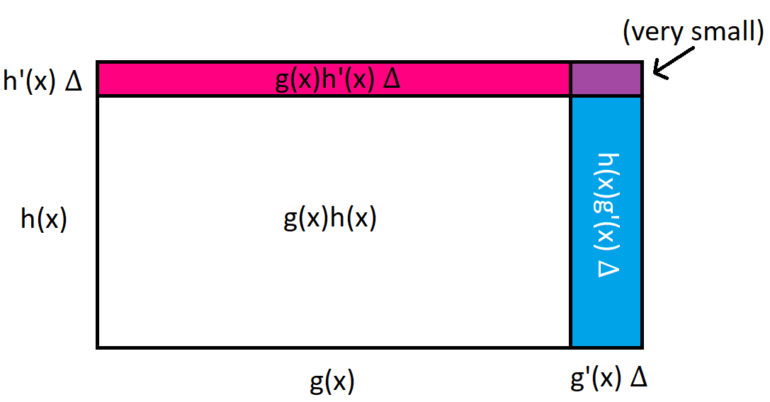
There’s a nice diagram that I can show you to try and illustrate this;

In the picture, there’s a rectangle with width $g(x)$ and height $h(x)$. The area is $g(x)h(x)$, which is the function $h(x)$ above. Here $x$ is an abstract variable, it’s not supposed to be anything to do with $x$-coordinates – just a sort of variable that’s controlling the width and height of this rectangle.
If that control variable changes by a little bit $\Delta$ (the Greek letter “delta” is often used for “change”), then the width of the rectangle increases by a little bit – roughly $g’(x)\Delta$. The height of the rectangle increases by roughly $h’(x)\Delta$. Each of those facts is really just what it means to be the derivative of $g(x)$ or $h(x)$.
The area of the rectangle increases with three different terms; there’s a pink area of size $g(x)h’(x)\Delta$, a blue area of size $g’(x)h(x)\Delta$ and a tiny purple area (its size is something to do with $\Delta^2$, and so if $\Delta$ is small then the purple area is much smaller than the blue or pink areas).
Overall then, the change in area when $x$ changes by $\Delta$ is something like $(g’(x)h(x)+g(x)h’(x))\Delta$. Said differently, the derivative is $g’(x)h(x)+g(x)h’(x)$.
Tangent planes
Some asked for more geometrical interpretation of partial derivatives, so here goes!
First, let’s quickly revisit some 1D theory. If you work out the derivative $f’(a)$ of a function $f(x)$ at some point $x=a$, then you can set up the tangent at that point as $y=f’(a)(x-a)+f(a)$. All I’ve done there is create a straight line $y=mx+c$ with the correct gradient, and the correct value when $x=a$. This gives us a tangent line for $f(x)$.
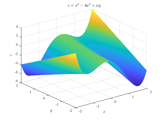
OK, let’s move to higher dimensions. For a function of two variables, we could plot this as a sort of surface in $(x,y,z)$-space, where the height $z=f(x,y)$ is the function. Here's a picture of $f(x,y)=x^4-4x^2+xy$.

The partial derivatives measure what happens when we change one variable and keep the other constant. Geometrically, this is like cutting a vertical plane through the surface and looking at the function in the slice. There are some pictures of what this looks like in the further reading for S1E7.
Let’s try and do something like that tangent line for this surface, at a point with $x=a$ and $y=b$, say. I suppose what we’re looking for now is higher dimensional – it’s a tangent plane rather than a tangent line. I’m going to jump to the equation and then explain it
$$z=f(a,b)+\left.\frac{\partial f}{\partial x}\right|_{(a,b)}(x-a) + \left.\frac{\partial f}{\partial y}\right|_{(a,b)}(y-b)$$
OK, so this is an equation for a plane – the constants are complicated, but if you squint at it you might be able to recognise the form $z=mx+ny+c$ for a plane. The idea is that this plane has the same $x$- and $y$- partial derivatives as the surface, just like how our tangent line above had the same (ordinary) derivative as the graph. The tangent plane gives us an approximation to the surface, which is handy for things like studying fluid dynamics on the surface of the Earth, where we might want to look at flow on the surface without worrying about the 3D positions of everything.
Why can’t I treat derivatives like fractions?
Here’s what happens in A-level; we’ve got something like $\frac{\mathrm{d}y}{\mathrm{d}x}=\text{stuff}$ and we want to write $\frac{\mathrm{d}x}{\mathrm{d}y}= 1/\text{stuff}$.
That’s actually fine for ordinary derivatives, where you’ve got a function of one variable. But let’s think about what it actually means. The derivative $\frac{dx}{dy}$ means something like “imagine $x$ is a function of $y$, write $x(y)$ and find the derivative with respect to $y$”. So really we’re doing something like finding the inverse function and differentiating.
Let me show you what happens for functions with more variables. Suppose we’ve got two functions $u(x,y)$ and $v(x,y)$. Then there are four partial derivatives that we could work out.
$$ \frac{\partial u}{\partial x}, \quad\frac{\partial u}{\partial y}, \quad\frac{\partial v}{\partial x}, \quad
\frac{\partial v}{\partial y}$$
If we somehow invert the equations to work out $x(u,v)$ and $y(u,v)$ (that could be really messy) and then differentiate them, then we’ve got four partial derivatives that we can work out
$$\frac{\partial x}{\partial u}, \quad\frac{\partial x}{\partial v}, \quad\frac{\partial y}{\partial u}, \quad
\frac{\partial y}{\partial v}$$
Now it would be great if each of those was just the reciprocal of one of the original ones. But the actual relationship between these eight things is more complicated (and much more interesting)
$$\left( \begin{matrix} \frac{\partial x}{\partial u}&\frac{\partial x}{\partial v}\\ \frac{\partial y}{\partial u}&\frac{\partial y}{\partial v} \end{matrix} \right) = \left( \begin{matrix} \frac{\partial u}{\partial x}&\frac{\partial u}{\partial y}\\ \frac{\partial v}{\partial x} &\frac{\partial v}{\partial y} \end{matrix} \right)^{-1}$$
So the real relationship between a derivative and the one that's "the other way up" involves a matrix inverse! For functions of one variable, we can get away with this without thinking about matrices, because 1-by-1 matrices behave just like numbers.
Curve sketching
If anyone’s still reading, here’s some curve sketching!
I’d like a graph of $y=\sin(x)-\sin(2x)$ and a graph of $y=\frac{1}{2}\sin(x)-\frac{1}{16}\sin(2x)$.
Have a go at sketching these (maybe put them into Desmos) and then comment on whether the following statement is true;
“For every value of $x$, the value of the second function is closer to zero than the value of the first function”.
If you want to get in touch with us about any of the mathematics in the video or the further reading, feel free to email us on oomc [at] maths.ox.ac.uk.

