Determination of University Standardised Marks
The Mathematics Teaching Committee issues each examination board with broad guidelines on the proportion of candidates that might be expected in the Distinction and the Merit classes. This is based on the average percentages in each class over the last four years, together with recent historic data for Part C, the MPLS Divisional averages, and the distribution of classifications achieved by the same group of students at Part B.
The examiners follow common practice in determining the University standardised marks (USMs) by using a scaling algorithm.
This year a new scaling algorithm was introduced to generate initial scaling maps in Part C, which removed the need to gauge the relative difficulty of papers by using previous year's marks of candidates as a baseline. Instead an in-year scaling was applied which compared papers by considering the average difference between each candidate’s raw mark on a given paper and their overall average raw mark across all standard papers.
Papers for which USMs are directly assigned by the markers or provided by another board of examiners are excluded from consideration. Calibration uses the Part C performance data of candidates in Mathematics and Mathematics & Statistics (Mathematics & Computer Science and Mathematics & Philosophy students are excluded at this stage).
The description below relates to the Part C examination, however the same process is used for Part B where Distinctions are replaced with First Classes and Merits are replaced with 2.1 Classes (and 64.5 and 65 is replaced by 59.5 and 60). Full marks in Part B can vary so the raw marks of 50 are instead replaced by $\mathrm{F}(P)$ — the full mark on paper $P$.
Piecewise-linear scaling maps
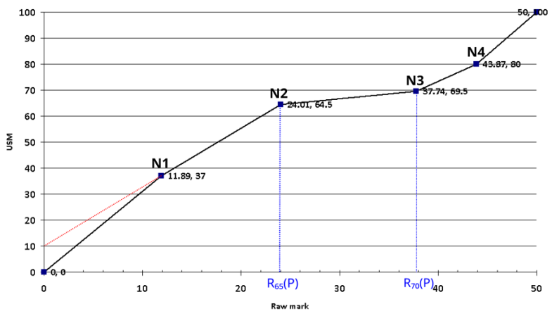
The goal is to produce a set of scaling maps $S_P: \rm{Raw} \to \rm{USM}$ for each paper $P$, where (generally) Raw $\in$ [0,50] is the raw mark, and USM $\in$ [0,100] is the University Standard Mark. We use piecewise-linear maps with five corners, with coordinates
(0,0), $N_1$=(c,37), $N_2$=$\left( R_{65}(P), 64.5 \right)$,$N_3$=$\left( R_{70}(P), 69.5 \right)$, $N_4$=$\left( \frac{50+R_{70}(P)}{2}, 80 \right)$, (50,100)
as shown in the example chart below.
Here $R_{65}(P)$ and $R_{70}(P)$ are the raw marks to be mapped to USM 64.5 and USM 69.5 and will be described below. The constant c is determined as follows: draw a straight line from $(0,10)$ to $N_2$, and then (c,37) is the point where this line meets the horizontal line y = 37. This is also illustrated in the figure below. The actual USMs are determined from $S_P(\rm{Raw})$ by symmetrically rounding to an integer. (This symmetrical rounding is why we chose 64.5 and 69.5 as y-coordinates above, as these are the actual Distinction/Merit and Merit/Pass borderlines.)

The scaling algorithm
The algorithm has two global inputs (independent of the paper), numbers $C_{70}$ and $C_{65}$, with $0<C_{70}+C_{65}<100$. To a first approximation, the algorithm aims to choose scaling maps such that $C_{70}$ percent of students $S$ get an average USM that satisfies $69.5 \leq \rm{AvUSM}(S) \leq 100$ (ie a Distinction) and the $C_{65}$ percent of candidates get $64.5 \leq \rm{AvUSM}(S) < 69.5$ (ie a Merit).
The Teaching Committee gives the examiners guidance each year on what proportions of each degree class to aim for, and this can be used to decide the values of $C_{70}$ and $C_{65}$.
We compute numbers $R_{70}$ and $R_{65}$ which are the lowest average raw marks for the top $C_{70}$ and $C_{70}+C_{65}$ percent of students in terms of their average raw mark. This is computed using all the standard mathematics and statistics papers taken together. If we defined piecewise-linear scaling maps by setting $R_{65}(P) = R_{65}$ and $R_{70}(P) = R_{70}$ for each paper $P$, then roughly $C_{70}$ percent of students would roughly expect to have an average USM of $69.5$ or above and a further $C_{65}$ percent of students would expect to have an average USM between $64.5$ and $69.5$, achieving the desired proportions of Distinctions and Merits.
The new algorithm then aims to account for the relative difficulty of papers. To do that we calculate a difficulty score on each paper $P$ (henceforth called $\mathrm{Diff}(P)$). We define $\mathrm{AvRaw}(S)$ to be the average raw mark for student $S$ over all the standard mathematics and statistics papers they took. We now define
\[
\mathrm{Diff}(P):=\mathrm{Av}_{S} (\mathrm{AvRaw}(S) - \mathrm{Raw}(P,S)),
\]
where the above average is over all Maths, OMMS and Maths & Stats students $S$ taking paper $P$.
In essence, raw marks in paper $P$ are $\mathrm{Diff}(P)$ lower than one would expect, given the cohort of students taking paper $P$. That is, $\mathrm{Diff}(P)$ is positive if the paper is harder, and negative if it is easier, so replacing $\mathrm{Raw}(P,S)$ by
\[
\mathrm{Raw'}(P,S):=\mathrm{Raw}(P,S)+\mathrm{Diff}(P)
\]
would, to a first approximation, adjust the marks to account for the difficulty this paper.
We hence define
\begin{eqnarray*}
R_{70}(P) &:=& R_{70} - \mathrm{Diff}(P) \\
R_{65}(P) &:=& R_{65} - \mathrm{Diff}(P)
\end{eqnarray*}
which determines nodes $N_2$ and $N_3$ of the piecewise linear function for paper $P$ at $N_2:=(R_{65}(P),64.5)$ and $N_3:=(R_{70}(P),69.5)$ in the piecewise-linear map described above.
Academic Judgement
A preliminary meeting of the internal examiners is held ahead of the examiners' meeting to assess the results produced by the algorithm alongside the reports from assessors. The examiners review each paper and assessors' reports, and discuss the preliminary scaling maps and the preliminary class percentage figures. The examiners have scope to make changes, usually by adjusting the position of the vertices $N_1,N_2,N_3,N_4$ by hand, so as to alter the $S_P$ map, to address any perceived unfairness introduced by the algorithm, particularly in cases with a small number of candidates. They also have the option to introduce additional vertices. Adjustments are made to the default settings as appropriate, paying particular attention to borderlines and to raw marks which were either very high or very low.

