High-Performance Low-Precision Vectorised Arithmetic and its Applications
 Researcher: Oliver Sheridan-Methven
- Academic Supervisor: Mike Giles
- Industrial Supervisor: Chris Goodyer
Background
Over the decades computers have become faster primarily through an increased density of transistors which can be fitted onto a chip, and the increased processing frequencies of CPUs. However, transistor density and clock frequencies are now reaching the maximum that can be manufactured, and so to improve performance new machines
are now built with ever increasing degrees of parallelism. Since the 1970's computers have been capable of a number of vector operations, and as part of the ever increasing on-chip parallelisation, many cores are returning to vector operations and hardware to perform several instructions in parallel, and hence achieve a greater computational throughput. This instruction level parallelism is known as vectorised arithmetic.
Furthermore, the trend over the past several decades has typically been to perform evermore precise computations, transitioning from single to double-precision. However, for several applications, even single-precision (corresponding to around 7 significant figures of accuracy) can be superfluous. For many applications where the level of precision can be reduced, then faster and slightly cruder algorithms can be implemented which are sufficient for the reduced precision. Examples which use lower-precision include graphics, machine learning, multilevel Monte Carlo, etc.
As computer hardware evolves a more developed set of instructions for handling vector operations, there are numerous technical considerations which need addressing to ensure programs fully utilise the computational resources and hardware capabilities. One of the first considerations is how best to reformat code so it can utilise the vector instruction set. Achieving this requires either a low-level knowledge of vector intrinsics, or a higher-level appreciation of writing algorithms which use single instruction multiple data (SIMD) operations. Re-writing algorithms in SIMD can be tricky, with several subtle or difficult caveats which need to be navigated, including: conditional branching, memory access patterns, etc. For applications which aim to utilise both the vector hardware and reduced precision, this can entail a total re-evaluation of which algorithms will achieve the best performance on a given machine.
Several branches of mathematics and their traditionally associated numeric schemes are readily ported onto modern hardware, and without any modification can directly reap the benefits of utilising the vector hardware or working in reduced precision. These branches of mathematics are fortunate. There are some branches of mathematics which keep the same performance as before. Even worse than this, there are some branches of mathematics whose performance can deteriorate from vectorised hardware and lower precisions. Random number generation, and consequently Monte Carlo methods, is an example of a branch of scientific calculation which is at risk of needlessly losing performance on modern hardware. The central focus of our research has been to investigate if we can not only remedy this problem, but fully exploit the capabilities of the new hardware.
Random Number Generation and Monte Carlo
The obvious question is why random number generation, and consequently Monte Carlo simulations, might suffer when performed on the latest hardware? (The common bottleneck in Monte Carlo simulations is usually the random number generation). To shed light on this we need to explain how computers generate random numbers following some given distribution. Consider then a few different types of distributions, which could include:
- The Bernoulli distribution (e.g. a coin toss).
- The discrete uniform distribution (e.g. the roll of a die).
- The continuous uniform distribution (e.g. an individual's height percentile)
- The Poisson distribution (e.g. waiting times of mechanical failure).
- The Gaussian distribution (e.g. average height of adults).
The typical building block for each of these computations is the discrete uniform distribution. The reason for this is that algorithms exist which can compute this very fast and to a high quality. Having a uniform distribution, we can generate most other distributions by interpreting the uniform value as a percentile of the distribution of interest. Then, seeing what value of the distribution would correspond to the given percentile gives us our desired random number. This is known as the inverse transformation method, and is a common and robust means of generating random numbers from any number of possible distributions. The popularity of the method stems in no small part
from its versatility.
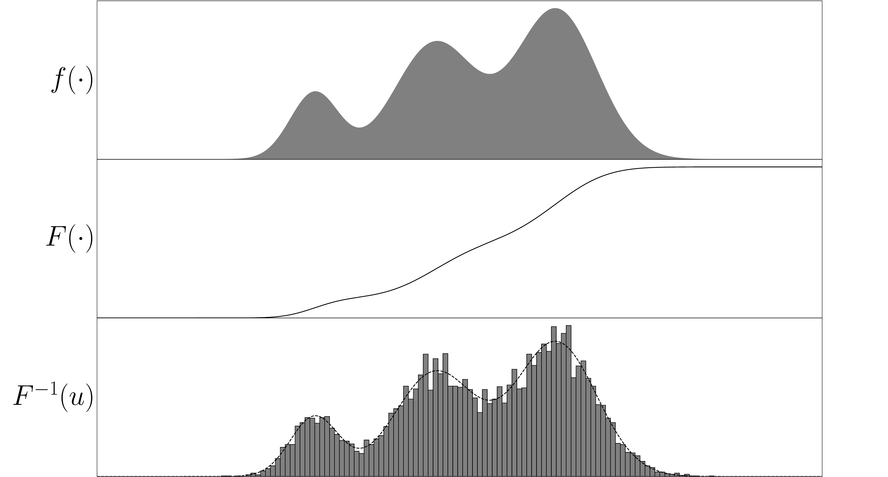
As an example of the scheme, suppose there is a probability distribution of interest. If we form the inverse cumulative distribution, and evaluate this for uniform random numbers between zero and one, then the output is exactly the desired distribution. An example of this is shown below.

Figure 1: The inverse transformation method: a distribution of interest (top), the cumulative distribution function (middle) and the inverse of the cumulative distribution evaluated for uniform random input between zero and one (bottom).
The Gaussian distribution, also known as the normal distribution, or the bell curve, is extremely ubiquitous and crucially important to many branches of mathematics, statistics, and science more widely. For this reason we have focused on how to speed up the inverse transformation method for the Gaussian distribution. Typical applications include understanding stock markets, or producing weather forecasts, among several others.
Outcomes
The outcome of our work has been to circumvent the expensive parts of the inverse transformation method, which especially manifest themselves when working on vectorised hardware and in reduced precision. The difficulty with the method is when we go into the tails of the distribution and need to calculate the rare-cases. To maintain accuracy in these more difficult calculations, the calculations are typically longer and more complicated. On vector hardware, and more so with reduced-precision, the greater the degree of parallelisation, it becomes a certainty that there will be a mix of mostly easy cases and some small number of more difficult tail cases. This requires the hardware to have to perform a mix of the two calculations, and having to do both of these results in the performance being poor for all the calculations. The situation only gets worse with greater parallelisation.
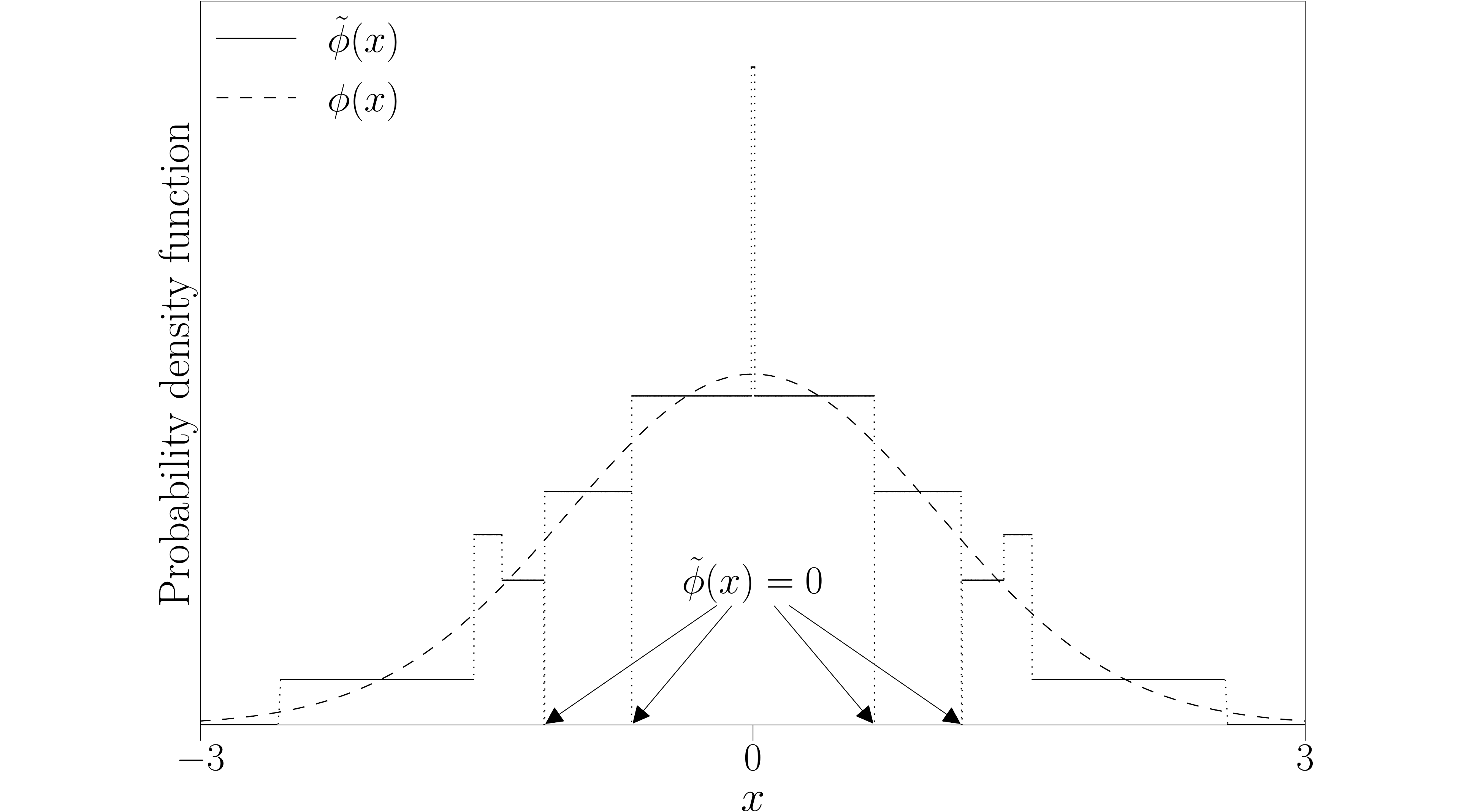
Our remedy to this was to construct approximations to the distribution which do not differentiate between the common calculations and the tail calculations. Rather the approximations are completely homogeneous in their design, construction, and implementation. Furthermore, the approximations are designed to be exceptionally fast on hardware. The key consequence of this is that you get random numbers which approximately follow the distribution you intended and have near identical statistics, but you get them much faster. This allows you to run simulations either in more detail or faster (or possibly both). An example of such an approximate distribution is shown below.

Figure 2: The Gaussian distribution and an approximate distribution. Although the approximation's probability density functions appears bizarre and not very good, inspecting the inverse cumulative distribution functions for these two, they match to a very high fidelity.
However, the approximate distribution being used and the exact distribution desired are slightly different. For high accuracy simulations, the discrepancy between the two distributions might be worrying. In our research, we have been able to quantify the discrepancy that switching to the approximate distributions incurs, and to relate this to the fidelity of our approximation, and thus control it if necessary. Furthermore, we can not only quantify this, but we can correct for this with only a marginal cost. (The procedure for making this correction that we developed and analysed was a nested multilevel Monte Carlo construction utilising a modified Euler-Maruyama scheme). The net result of this is that we are able to run complex simulations at a greatly reduced cost (e.g. in only 20% of the original time), but without losing any of the accuracy! Coupling this with the rigour of the mathematical proofs, this allows practitioners to be confident they are getting the right answers.

